L'usage de la calculatrice avec mode examen actif est autorisé.
L'usage de la calculatrice sans mémoire "type collège" est autorisé.
Sauf mention contraire, toute réponse devra être justifiée.
Le candidat est invité à faire figurer sur la copie toute trace de recherche, même
La qualité de la rédaction, la clarté et la précision des raisonnements seront prises en
compte dans l'appréciation de la copie. Les traces de recherche, même incomplètes
ou infructueuses seront valorisées.
5 points
exercice 1
Thèmes : probabilités, suites
5 points
exercice 2
Thème : Géométrie dans l'espace
5 points
exercice 3
Thème : étude de fonctions
5 points
exercice 4
Thème : suites, fonction logarithme, algorithmique
Bac général spécialité maths 2023 -Polynésie jour 2
Partager :
5 points
exercice 1
Thèmes : probabilités, suites
Partie A
Chaque jour, un athlète doit sauter une haie en fin d'entraînement. Son entraîneur estime, au vu de la saison précédente, que :
si l'athlète franchit la haie un jour, alors il la franchira dans90 % des cas le jour suivant; si l'athlète ne franchit pas la haie un jour, alors dans 70 % des cas, il ne la franchira pas non plus le lendemain.
1. Arbre pondéré complété.
2. En nous aidant de l'arbre, nous déduisons que :
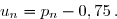
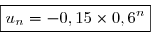
3. On considère la suite (un ) définie, pour tout entier naturel n , par :
3. a) Démontrons que la suite (un ) est géométrique.
Pour tout entier naturel n ,
Par conséquent, la suite (un ) est une suite géométrique de raison q = 0,6 dont le premier terme est u0 = -0,15.
3. b) Le terme général de la suite (un ) est
Donc, pour tout entier naturel n ,
Dès lors,
3. c) Nous devons calculer
3. d) A long terme, après un grand nombre d'entraînements, l'athlète réussira à franchir la haie avec une probabilité d'environ 0,75 c'est-à-dire environ 3 fois sur 4.
Partie B
1. Lors de cette expérience, on répète 10 fois des épreuves identiques et indépendantes.
Chaque épreuve comporte deux issues :
Succès : « la haie a été franchie par l'athlète à l'issue d'un 400 mètres haies » dont la probabilité est p = 0,75.
Echec : « la haie n'a pas été franchie par l'athlète à l'issue d'un 400 mètres haies » dont la probabilité est 1 - p = 1 - 0,75 = 0,25.
La variable aléatoire X compte le nombre de haies franchies par l'athlète à l'issue d'un 400 mètres haies, soit le nombre de succès à la fin de la répétition des épreuves.
D'où la variable aléatoire X suit une loi binomiale .
Cette loi est donnée par :
2. Déterminons la probabilité que l'athlète franchisse les 10 haies, soit P (X = 10).
Par conséquent, la probabilité que l'athlète franchisse les 10 haies est environ égale à 0,056 (valeur arrondie à 10-3 près)
3. Nous devons calculer P (X 9).
Par conséquent, la probabilité que, à l'issue d'un 400 mètres haies, l'athlète ait franchi au moins 9 d'entre elles est environ égale à 0,244.
5 points
exercice 2
Thème : Géométrie dans l'espace
L'espace est muni d'un repère orthonormé
On considère :
le point A (1 ; -1 ; -1) ; le plan d'équation : ; le plan d'équation : ; la droite de représentation paramétrique :
1. Montrons que les plans et ne sont pas parallèles.
Nous savons que tout plan dont l'équation cartésienne est de la forme : ax + by + cz + d = 0, admet un vecteur normal .
Dès lors, un vecteur normal au plan est et un vecteur normal au plan est .
Les vecteurs et ne sont pas colinéaires.
En effet,
Par conséquent, les plans et ne sont pas parallèles.
2. Démontrons que est la droite d'intersection de et
Montrons que tout point de la droite appartient au plan Montrons donc que la représentation paramétrique de vérifie l'équation de
Pour tout réel t , nous obtenons :
D'où, tout point de appartient au plan et par suite, la droite est incluse au plan
De même, montrons que tout point de la droite appartient au plan Montrons donc que la représentation paramétrique de vérifie l'équation de
Pour tout réel t , nous obtenons :
D'où, tout point de appartient au plan et par suite, la droite est incluse au plan
En conclusion, la droite est incluse dans les deux plans non parallèles et
Par conséquent, est la droite d'intersection de et
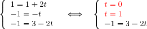
3. a) Montrons que le point A n'appartient pas à en montrant que ses coordonnées ne vérifient pas l'équation de
En effet,
3. b) Montrons que le point A n'appartient pas à en montrant que ses coordonnées ne vérifient pas la représentation paramétrique de
En effet,
Ce système étant impossible, nous en déduisons que le point A n'appartient pas à
4. Pour tout réel t , on note M le point de de coordonnées
On considère alors la fonction f qui à tout réel t associe AM2, soit
4. a) Pour tout réel t ,
4. b) Utilisons le fait que AM est minimale si et seulement si AM2 est minimale.
La fonction f est une fonction du second degré possédant un minimum car le coefficient principal est 9 > 0.
Ce minimum est atteint pour
Dans ce cas, les coordonnées du point M sont
Par conséquent, la distance AM est minimale lorsque M a pour coordonnées (3 ; -1 ; 1).
5. On note H le point de coordonnées (3 ; -1 ; 1). Démontrons que la droite (AH ) est perpendiculaire à
Le point H de coordonnées (3 ; -1 ; 1) coïncide avec le point M défini dans la question 4. et tel que la distance AM est minimale.
Nous en déduisons que le point H est la projection orthogonale du point A sur la droite
Par conséquent, la droite (AH ) est perpendiculaire à
5 points
exercice 3
Thème : étude de fonctions
Partie A
Le plan est ramené à un repère orthogonal.
On a représenté ci-dessous la courbe d'une fonction f définie et deux fois dérivable sur R, ainsi que celle de sa dérivée f' et de sa dérivée seconde f'' .
1. Notons la fonction représentée par la courbe , la fonction représentée par la courbe et la fonction représentée par la courbe
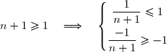
Graphiquement, nous observons que est strictement croissante alors que est strictement positive sur R.
Nous en déduisons que
De plus, est strictement croissante sur ]- ; 4[ et strictement décroissante sur ]4 ; +[ alors que est strictement positive sur ]- ; 4[ et strictement négative sur ]4 ; +[.
Nous en déduisons que
D'où
Par conséquent, la fonction f'' est représentée par la courbe , la fonction f' est représentée par et la fonction f est représentée par
2. Nous devons déterminer le coefficient directeur de la tangente à la courbe au point d'abscisse 4.
Si nous adoptons les notations définies dans la question précédente, nous devons donc déterminer , soit
Avec la précision permise par le graphique, nous observons que
Donc le coefficient directeur de la tangente à la courbe au point d'abscisse 4 est égal à 3.
3. Avec la précision permise par le graphique, nous observons que les abscisses des points d'inflexion de la courbe sont approximativement égales à 3,1 ; 4 et 4,9.
Partie B
Soit un réel k strictement positif.
On considère la fonction g définie sur R par :
1. Nous devons déterminer les limites de g en + et -.
Calculons
Il s'ensuit que
Calculons
Il s'ensuit que
2. Nous devons prouver que
La fonction g est dérivable sur R.
Pour tout x réel,
3. Selon l'énoncé, nous admettons que
Étudions le signe de g'' (x ) sur R.
La dérivée seconde s'annule en 0 en y changeant de signes.
Par conséquent, la courbe représentative de la fonction g possède un unique point d'inflexion au point d'abscisse 0.
5 points
exercice 4
Thèmes : suites, fonction logarithme, algorithmique
Affirmation 1 : "La suite u définie pour tout entier naturel n par est bornée". Affirmation vraie.
En effet, nous savons que
Dès lors, nous avons :
Pour tout entier naturel n , nous obtenons alors :
De plus,
En résumé, nous obtenons :
et donc, pour tout entier naturel n ,
Par conséquent, la suite u est bornée (minorée par -1 et majorée par 1).
Donc l'affirmation 1 est vraie.
Affirmation 2 : "Toute suite bornée est convergente". Affirmation fausse.
Un contre-exemple est donné par la suite u définie pour tout entier naturel n par .
Cette suite est bornée par -1 et 1 et n'est pas convergente puisque ses termes valent alternativement -1 et 1.
Donc l'affirmation 2 est fausse.
Affirmation 3 : "Toute suite croissante tend vers +". Affirmation fausse.
Un contre-exemple est donné par la suite u définie pour tout entier naturel non nul n par .
Montrons que cette suite est croissante.
Pour tout entier naturel non nul n ,
Nous en déduisons que la suite u est strictement croissante.
Cette suite ne tend pas vers + car
Par conséquent, tout suite croissante ne tend pas nécessairement vers +.
Donc l'affirmation 3 est fausse.
Soit la fonction f définie sur R par Affirmation 4. : "La fonction f est convexe sur l'intervalle [-3 ; 1]". Affirmation fausse.
Étudions le signe de la dérivée seconde f''.
Étudions le signe de g'' (x ) sur R.
Nous observons que la dérivée seconde change de signe en x = -2 et x = 0.
Il s'ensuit que la fonction f change de concavité en x = -2 et x = 0.
Or les valeurs 0 et 2 appartiennent à l'intervalle [-3 ; 1].
Par conséquent, la fonction f n'est pas convexe sur tout l'intervalle [-3 ; 1].
Donc l'affirmation 4 est fausse.
On considère la fonction mystere définie ci-dessous qui prend une liste L de nombres en paramètre.
Affirmation 5. : "L'exécution de mystère([2,3,7,0,6,3,2,0,5]) renvoie 7." Affirmation vraie.
En effet, la fonction mystere renvoie le maximum de la liste L qui est bien 7.
Donc l'affirmation 5 est vraie.
Publié par malou
le
ceci n'est qu'un extrait
Pour visualiser la totalité des cours vous devez vous inscrire / connecter (GRATUIT) Inscription Gratuitese connecter
Merci à Hiphigenie / malou pour avoir contribué à l'élaboration de cette fiche
Désolé, votre version d'Internet Explorer est plus que périmée ! Merci de le mettre à jour ou de télécharger Firefox ou Google Chrome pour utiliser le site. Votre ordinateur vous remerciera !
 si l'athlète franchit la haie un jour, alors il la franchira dans90 % des cas le jour suivant;

 \\ \overset{ { \white{ . } } } { \phantom{ p_{ n+1 } } = p_n\times0,9+(1-p_n)\times0,3 } \\ \overset{ { \white{ . } } } { \phantom{ p_{ n+1 } } = 0,9\,p_n+0,3-0,3\,p_n } \\ \overset{ { \white{ . } } } { \phantom{ p_{ n+1 } } = 0,6\,p_n+0,3 } \\ \\ \Longrightarrow\boxed{ p_{n+1}=0,6\,p_n+0,3 })

-0,75 } \\ \overset{ { \white{ . } } }{ \phantom{ u_{ n+1 } }=0,6p_n-0,45 } \\ \overset{ { \phantom{ . } } }{ \phantom{ u_{ n+1 } }=0,6p_n-0,6\times0,75 } \\ \overset{ { \white{ . } } }{ \phantom{ u_{ n+1 } }=0,6(p_n-0,75) } \\ \overset{ { \phantom{ . } } }{ \phantom{ u_{ n+1 } }=0,6u_n } \\ \\ \Longrightarrow\boxed{ \forall\ n\in\N, \ u_{ n+1 }=0,6u_n } )


=0,75 } \\ \\ \text{ D'où }\;\boxed{ \ell=\lim\limits_{ n\to+\infty }p_n=0,75 }\,.)
 }) .
.=\begin{pmatrix}10\\k\end{pmatrix}\times0,75^k\times0,25^{ 10-k } })
=\begin{pmatrix}10\\10\end{pmatrix}\times0,75^{ 10 }\times0,25^{ 10-10 } \\ \overset{ { \white{ . } } }{ \phantom{ P(X=10) }=1\times0,75^{ 10 }\times1 } \\ \overset{ { \white{ . } } }{ \phantom{ P(X=10) }=0,75^{ 10 } } \\ \overset{ { \white{ . } } }{ \phantom{ P(X=10) }\approx0,056 } \\ \\ \Longrightarrow\quad\boxed{ P(X=10)=0,75^{ 10 }\approx0,056 })
 9).
9).=P(X=9)+P(X=10) \\ \overset{ { \white{ . } } }{ \phantom{ P(X\ge9) }=\begin{pmatrix}10\\9\end{pmatrix}\times0,75^9\times0,25^{ 10-9 }+0,75^{10}} \\ \overset{ { \phantom{ . } } }{ \phantom{ P(X\ge9) }= 10\times0,75^9\times0,25+0,75^{10}} \\ \overset{ { \white{ . } } }{ \phantom{ P(X\ge9) }\approx0,244 } \\ \\ \Longrightarrow\quad\boxed{ P(X\ge9)\approx0,244 })
.)
 d'équation :
  ;
; d'équation :
 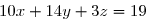 ;
; de représentation paramétrique :
  )
 .
. et un vecteur normal au plan
  .
. et
et  ne sont pas colinéaires.
 )

 Montrons que tout point de la droite
+2(-t)+4(3-2t)=5+10t-2t+12-8t=17. })

+14(-t)+3(3-2t)=10+20t-14t+9-6t=19. })

+4\times(-1)=5-2-4=-1\neq17. })

 \,.})
=AM^2. })

-1\\ \overset{ { \white{ . } } }{ -t-(-1) } \\ \overset{ { \white{ . } } }{ 3-2t-(-1) }\end{pmatrix}=\begin{pmatrix}2t\\ \overset{ { \white{ . } } }{1 -t }\\ \overset{ { \phantom{ . } } }{ 4-2t }\end{pmatrix} \\ \\ \\ \Longrightarrow\quad f(t)=AM^2 \\ \overset{ { \phantom{ . } } }{ \phantom{ WWWW }=(2t)^2+(1-t)^2+(4-2t)^2 } \\ \overset{ { \phantom{ . } } }{ \phantom{ WWWW }=4t^2+1-2t+t^2+16-16t+4t^2} \\ \overset{ { \phantom{ . } } }{ \phantom{ WWWW }=9t^2-18t+17 } \\ \\ \Longrightarrow\quad\boxed{ f(t)=9t^2-18t+17 })
 }{2\times9}=1\,. })
 }=(3\;;\;-1\;;\;1)\,.)
 la fonction représentée par la courbe
  ,
,  la fonction représentée par la courbe
  et
et  la fonction représentée par la courbe

 ; 4[ et strictement décroissante sur ]4 ; +

 et la fonction f est représentée par
 }) , soit
, soit \,. })
\approx3\,. })
=\dfrac{ 4 }{ 1+\text e^{ -kx } }\;. })
 Calculons
 . })
=-\infty \\ \overset{ { \white{ . } } }{ \lim\limits_{ X\to-\infty }\text{ e }^X=0\phantom{ W } }\end{matrix}\right.\quad\underset{ (X=-kx) }{ \Longrightarrow }\quad\lim\limits_{ x\to+\infty }\text{ e }^{ -kx }=0 \\ \phantom{ WWWWWWvWWWW }\Longrightarrow\quad\quad\lim\limits_{ x\to+\infty }(1+\text{ e }^{ -kx })=1 \\ \\ \phantom{ WWWWWWvWWWW }\Longrightarrow\quad\quad\lim\limits_{ x\to+\infty }\dfrac{ 4 }{ 1+\text e^{ -kx } }=\dfrac{ 4 }{ 1 }=4)
=4 }. })
. })
=+\infty \\ \overset{ { \white{ . } } }{ \lim\limits_{ X\to+\infty }\text{ e }^X=+\infty\phantom{ W } }\end{matrix}\right.\quad\underset{ (X=-kx) }{ \Longrightarrow }\quad\lim\limits_{ x\to-\infty }\text{ e }^{ -kx }=+\infty \\ \phantom{ WWWWWWvWWWW }\Longrightarrow\quad\quad\lim\limits_{ x\to-\infty }(1+\text{ e }^{ -kx })=+\infty \\ \\ \phantom{ WWWWWWvWWWW }\Longrightarrow\quad\quad\lim\limits_{ x\to-\infty }\dfrac{ 4 }{ 1+\text e^{ -kx } }=0)
=0 }. })
=k. })
=4\times\left(\dfrac{ 1 }{ 1+\text e^{ -kx } }\right)' } \\ \overset{ { \white{ . } } } { \phantom{ g'(x) }=4\times\dfrac{ -(1+\text e^{ -kx })' }{ (1+\text e^{ -kx })^2 } } \\ \overset{ { \white{ . } } } { \phantom{ g'(x) }=4\times\dfrac{ -(-k)\,\text e^{ -kx } }{ (1+\text e^{ -kx })^2 } } \\ \overset{ { \white{ . } } } { \phantom{ g'(x) }=\dfrac{ 4k\,\text e^{ -kx } }{ (1+\text e^{ -kx })^2 } } \\ \\ \Longrightarrow \boxed{g'(x)=\dfrac{ 4k\,\text e^{ -kx } }{ (1+\text e^{ -kx })^2 } })
=\dfrac{ 4k\,\text e^{ 0 } }{ (1+\text e^{ 0 })^2 }=\dfrac{ 4k\times1 }{ (1+1)^2 }=\dfrac{ 4k }{ 4 }=k \\ \\ \quad\Longrightarrow\quad\boxed{ g'(0)=k })
=-4\,\text e^{ kx }\,(\text e^{ kx }-1)\,\dfrac{ k^2}{\left(\text e^{ kx }+1\right)^3}\,. })
^3&&+&&+&&+&\\&&&&&&&\\ \hline&&&&&&&\\g''(x)&&+&&0&&-&\\&&&& &&&\\ \hline \end{array})
^n }{ n+1 }) est bornée".
est bornée". Affirmation vraie.
^n=\left\lbrace\begin{matrix}-1\quad\text{ si }n\text{ est impair }\\1\quad\text{ si }n\text{ est pair }\end{matrix}\right. })
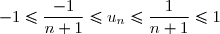
^n\le 1.)
^n\le 1\quad\Longrightarrow\quad \dfrac{ -1 }{ n+1 } \le \dfrac{ (-1)^n } { n+1 } \le \dfrac{ 1 } { n+1 } \\ \overset{ { \white{ . } } } {\phantom{WWWWWWw }\quad\Longrightarrow\quad \dfrac{ -1 }{ n+1 } \le u_n \le \dfrac{ 1 } { n+1 } })
^n) .
. .
. \\ \overset{ { \white{ . } } } { \phantom{u_{ n+1 }-u_n }=-\dfrac{ 1 }{ n+1 }+\dfrac{ 1 }{ n } } \\ \overset{ { \white{ . } } } { \phantom{u_{ n+1 }-u_n }=\dfrac{ -n+n+1 }{ n(n+1) } } \\ \overset{ { \white{ . } } } { \phantom{u_{ n+1 }-u_n }=\dfrac{ 1 }{ n(n+1) } } \\ \\ \Longrightarrow\boxed{ u_{n+1}-u_n=\dfrac{ 1 }{ n(n+1) }>0\quad(\text{car }n>0) })

=\ln(x^2+2x+2).)
=\left(\overset { } { \ln(x^2+2x+2) } \right)' \\ \overset{ { \white{ . } } } { \phantom{f'(x) }= \dfrac{ (x^2+2x+2)' } { x^2+2x+2 } } \\ \overset{ { \white{ . } } } { \phantom{f'(x) }= \dfrac{ 2x+2 } { x^2+2x+2 } } \\ \\ \Longrightarrow\boxed{ f'(x)= \dfrac{ 2x+2 } { x^2+2x+2 } })
= \left(\dfrac{ 2x+2 } { x^2+2x+2 }\right)' \\ \overset{ { \white{ . } } } { \phantom{f''(x) }= \dfrac{ (2x+2)'\times(x^2+2x+2)-(2x+2)\times(x^2+2x+2)' } { (x^2+2x+2)^2 } } \\ \overset{ { \white{ . } } } { \phantom{f''(x) }= \dfrac{ 2\times(x^2+2x+2)-(2x+2)\times(2x+2) } { (x^2+2x+2)^2 } } \\ \overset{ { \white{ . } } } { \phantom{f''(x) }= \dfrac{ (2x^2+4x+4)-(4x^2+8x+4) } { (x^2+2x+2)^2 } } \\ \overset{ { \phantom{ . } } } { \phantom{f''(x) }= \dfrac{ -2x^2-4x} { (x^2+2x+2)^2 } } \\ \\ \Longrightarrow\boxed{ f''(x)= \dfrac{ -2x^2-4x} { (x^2+2x+2)^2 } })
=0 \\ \phantom{ WWWWWWWW }\Longleftrightarrow-2x=0\text{ ou }x+2=0\\ \phantom{ WWWWWw }\Longleftrightarrow x=0\text{ ou }x=-2\end{matrix}\phantom{ W } \begin{matrix}|\\|\\|\\|\\|\\|\\|\\|\\|\end{matrix}\phantom{ W }\begin{array} { |c|cccccccc| } \hline &&&&&&&&& x &-\infty&&-2&&0&&&+\infty\\ &&&&&&&& \\ \hline&&&&&&&& \\ -2x^2-4x&& - &0&+&0& - &&\\ (x^2+2x+2)^2&&+&+&+&+&+&&\\&&&&&&&&\\ \hline&&&&&&&&\\f''(x)&&-&0&+&0&-&&\\&&&&& &&&\\ \hline \end{array})
![{\white{WWWWW}}\begin{array} { |l|l| } \hline { \blue { \text{d} } } { \blue { \text{e} } } { \blue { \text {f} } } \text{ mystere(L)} :\phantom{ Wwx } \\ \phantom{ Wii }\text{M = L}[0]\phantom{ Wwww } \\ \phantom{ Wii }\sharp\text{On initilaise M avec le premier élément de la liste L} \\ \phantom{ x }\phantom{ w } { \blue { \text{ for } } }\text{ i in range(len(L))}:\phantom { Wi } \\ \phantom { x } \phantom { WWvi }{ \blue { \text{ if } } }\text{ L}[\text{i}] >\text{ M :}\phantom { W XWxi } \\ \phantom { x } \phantom { WWWWvi } \text{ M = \text{ L}[\text{i}]}\phantom { W XWxi } \\ \phantom { x } \phantom { w } { \blue { \text { return } } } { \text { M } } \phantom { Wi } \\ \hline\end {array}](https://latex.ilemaths.net/latex-0.tex?{\white{WWWWW}}\begin{array} { |l|l| } \hline { \blue { \text{d} } } { \blue { \text{e} } } { \blue { \text {f} } } \text{ mystere(L)} :\phantom{ Wwx } \\ \phantom{ Wii }\text{M = L}[0]\phantom{ Wwww } \\ \phantom{ Wii }\sharp\text{On initilaise M avec le premier élément de la liste L} \\ \phantom{ x }\phantom{ w } { \blue { \text{ for } } }\text{ i in range(len(L))}:\phantom { Wi } \\ \phantom { x } \phantom { WWvi }{ \blue { \text{ if } } }\text{ L}[\text{i}] >\text{ M :}\phantom { W XWxi } \\ \phantom { x } \phantom { WWWWvi } \text{ M = \text{ L}[\text{i}]}\phantom { W XWxi } \\ \phantom { x } \phantom { w } { \blue { \text { return } } } { \text { M } } \phantom { Wi } \\ \hline\end {array} )
 Voir la correction
 forum de terminale