L'usage de la calculatrice avec mode examen actif est autorisé.
L'usage de la calculatrice sans mémoire, « type collège » est autorisé.
Le candidat est invité à faire figurer sur la copie toute trace de recherche, même
incomplète ou non fructueuse, qu'il aura développée.
La qualité de la rédaction, la clarté et la précision des raisonnements seront prises en
compte dans l'appréciation de la copie. Les traces de recherche, même incomplètes ou
infructueuses seront valorisées.
5 points
exercice 1 : QCM
Cet exercice est un questionnaire à choix multiples. Pour chaque question, une seule
des quatre propositions est exacte. Indiquer sur la copie le numéro de la question et
la lettre de la proposition choisie. Aucune justification n'est demandée.
Pour chaque question, une réponse exacte rapporte un point. Une réponse fausse,
une réponse multiple ou l'absence de réponse ne rapporte ni n'enlève de point.
1. Soit f la fonction définie sur par
Une primitive F , définie sur de la fonction f est définie par
La fonction F est dérivable sur (produit de deux fonctions dérivables sur ).
Pour tout
Par conséquent, une primitive de la fonction f , définie sur par est la fonction F , définie sur par
Donc la réponse B est correcte.
2. La courbe C ci-dessous représente une fonction f définie et deux fois dérivable sur ]0 ; +[.
On sait que :
le maximum de la fonction f est atteint au point d'abscisse 3 ; le point P d'abscisse 5 est l'unique point d'inflexion de la courbe C .
On a : pour tout x ]5 ; +[, f (x ) et f'' (x ) sont de même signe
En effet, nous observons graphiquement que sur l'intervalle ]5 ; +[, et également que la fonction f est convexe, soit
Par conséquent, pour tout x ]5 ; +[, f (x ) et f'' (x ) sont de même signe.
Donc la réponse D est correcte.
3. On considère la fonction g définie sur ]0 ; +[ par où a et b sont deux nombres réels.
On sait que et Les valeurs de a et b sont a = 6 et b = 2
Par conséquent, les valeurs de a et b sont a = 6 et b = 2.
Donc la réponse D est correcte.
4. Sachant qu'Alice a tiré une boule verte, la probabilité qu'elle ait choisi l'urne B est égale à
Soit les événements A : '' l'urne A est choisie '' et B : '' l'urne B est choisie ''
ainsi que les événements V : '' la boule tirée est verte '' et R : '' la boule tirée est rouge ''.
Ci-dessous, un arbre pondéré représentant les données du problème.
Nous devons calculer
Calculons d'abord
Les événements et forment une partition de l'univers.
En utilisant la formule des probabilités totales, nous obtenons :
Dès lors,
D'où sachant qu'Alice a tiré une boule verte, la probabilité qu'elle ait choisi l'urne B est égale à
Donc la réponse C est correcte.
5. On pose
Parmi les scripts Python ci-dessous, celui qui permet de calculer la somme S est le script b.
En effet, le script "a" permet de calculer chaque terme de la somme. Par contre, il ne calcule pas cette somme.
le script "c" permet de calculer la somme des termes tant que cette somme est inférieure à 100. Cela ne correspond pas à ce qui est demandé.
le script "d" propose une boucle qui ne s'arrêtera jamais puisque la valeur de k ne change pas lors de chaque passage.
Donc la réponse b. est correcte.
6 points
exercice 2
On considère la fonction f définie sur ]-1,5 ; +[ par
Nous allons étudier la convergence de la suite (un ) définie par : et pour tout entier naturel n .
Partie A : Étude d'une fonction auxiliaire
On considère la fonction g définie sur ]-1,5 ; +[ par
1. Calculons
Il s'ensuit que
On admet que
2. Nous devons étudier les variations de la fonction g sur ]-1,5 ; +[.
La fonction g est dérivable sur ]-1,5 ; +[.
Pour tout réel x ]-1,5 ; +[,
Étudions le signe de g' (x ) et les variations de g sur ]-1,5 ; +[.
Par conséquent, la fonction g est strictement croissante sur l'intervalle ]-1,5 ; -0,5] et strictement décroissante sur l'intervalle [-0,5 ; +[.
3. a) Montrons que, dans l'intervalle ]-0,5 ; +[, l'équation g (x ) = 0 admet une unique solution .
La fonction g est continue sur l'intervalle ]-0,5 ; +[ car elle est dérivable sur cet intervalle.
La fonction g est strictement décroissante sur l'intervalle ]-0,5 ; +[.
Selon le corollaire du théorème des valeurs intermédiaires, il existe un unique réel appartenant à ]-0,5 ; +[ tel que
3. b)
Partie B : Étude de la suite (un )
On admet que la fonction f est strictement croissante sur ]-0,5 ; +[.
1. Soit x un nombre réel. Montrons que si alors
En effet,
Par conséquent, si alors
2. a) Nous devons montrer par récurrence que, pour tout entier naturel n :
Initialisation : Montrons que la propriété est vraie pour n = 0, soit que
C'est une évidence car
Donc l'initialisation est vraie.
Hérédité : Montrons que si pour un nombre naturel n fixé, la propriété est vraie au rang n , alors elle est encore vraie au rang (n +1).
Montrons donc que si pour un nombre naturel n fixé, , alors
En effet,
D'où l'hérédité est vraie.
Puisque l'initialisation et l'hérédité sont vraies, nous avons montré par récurrence que
2. b) Nous avons montré dans la question précédente que la suite (un ) est croissante et majorée par .
Selon le théorème de convergence monotone, nous en déduisons que la suite (un ) est convergente.
6 points
exercice 3
La figure ci-dessous correspond à la maquette d'un projet architectural.
Il s'agit d'une maison de forme cubique (ABCDEFGH ) accolée à un garage de forme cubique (BIJKLMNO ) où L est le milieu du segment [BF ] et K le milieu du segment [BC ].
Le garage est surmonté d'un toit de forme pyramidale (LMNOP ) de base carrée LMNO et de sommet P positionné sur la façade de la maison.
On munit l'espace d'un repère orthonormé avec
1. a) Par lecture graphique, nous obtenons :
1. b) Déterminons une représentation paramétrique de la droite (HM ).
La droite (HM ) est dirigée par le vecteur .
Donc la droite (HM ) est dirigée par le vecteur
La droite (HM ) passe par le point
D'où une représentation paramétrique de la droite (HM ) est donnée par :
soit
2. L'architecte place le point P à l'intersection de la droite (HM ) et du plan (BCF ).
Déterminons les coordonnées de P .
Une équation du plan (BCF ) est car les abscisses des points B, C et F sont égales à 2.
Soit les coordonnées du point P .
Le point P appartient à la droite (HM ) et au plan (BCF ).
Dès lors, est solution du système suivant que nous résolvons :
Par conséquent, les coordonnées de P sont
3. a) Nous devons calculer le produit scalaire
3. b) Nous devons calculer la distance PM .
On admet que
3. c) Déterminons l'amplitude de l'angle
En utilisant les résultats des réponses précédentes, nous obtenons :
Par conséquent, le toit pourra être construit car l'angle ne dépasse pas 55°.
4. Nous devons justifier que les droites (HM ) et (EN ) sont sécantes.
Déterminons une représentation paramétrique de la droite (EN ).
La droite (EN ) est dirigée par le vecteur .
Donc la droite (EN ) est dirigée par le vecteur
La droite (EN ) passe par le point
D'où une représentation paramétrique de la droite (EN ) est donnée par :
soit
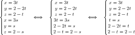
Les droites (HM ) et (EN ) sont sécantes si le système composé des représentations paramétriques de ces droites possède une solution.
Résolvons ce système.
Nous en déduisons que les droites (HM ) et (EN ) sont sécantes en
3 points
exercice 4
Lors de cette expérience, on répète 4 fois des épreuves identiques et indépendantes.
Chaque épreuve comporte deux issues :
Succès : « le candidat est qualifié » dont la probabilité est p = 0,6
Echec : « le candidat n'est pas qualifié » dont la probabilité est 1 - p = 0,4.
Soit la variable aléatoire X comptant le nombre de candidats qualifiés parmi les quatre candidats, soit le nombre de succès à la fin de la répétition des épreuves.
La variable aléatoire X suit alors une loi binomiale .
Cette loi est donnée par :
Dès lors,
Résumons cette loi de probabilité dans un tableau.
Vérifions si la condition n°1 est vérifiée, soit si
Par conséquent, la condition n°1 est vérifiée.
Vérifions si la condition n°2 est vérifiée.
Déterminons la durée moyenne de la deuxième phase.
Soit la variable aléatoire T exprimant la durée de la deuxième phase en minutes.
Reprenons le tableau donné dans l'énoncé.
Calculons l'espérance mathématique de la variable aléatoire T .
Nous observons alors que
Par conséquent, la condition n°2 n'est pas vérifiée.
Comme les deux conditions ne sont pas vérifiées, il s'ensuit que le jeu ne pourra pas être retenu.
Publié par malou
le
ceci n'est qu'un extrait
Pour visualiser la totalité des cours vous devez vous inscrire / connecter (GRATUIT) Inscription Gratuitese connecter
Merci à Hiphigenie / malou pour avoir contribué à l'élaboration de cette fiche
Désolé, votre version d'Internet Explorer est plus que périmée ! Merci de le mettre à jour ou de télécharger Firefox ou Google Chrome pour utiliser le site. Votre ordinateur vous remerciera !
 par
par =x\,\text{e}^x\,. })
=(x-1)\,\text e^x}\quad {\red{\longrightarrow\quad\text{Réponse B.}}})


=(x-1)'\times\text e^x+(x-1)\times(\text e^x)' \\ \overset{ { \white{ . } } } { \phantom{F\,'(x)}=1\times\text e^x+(x-1)\times \text e^x } \\ \overset{ { \white{ . } } } { \phantom{F\,'(x)}=(1+x-1)\, \text e^x } \\ \overset{ { \white{ . } } } { \phantom{F\,'(x)}=x\, \text e^x })
}=f(x)} \\ \\ \Longrightarrow\quad \boxed{ \forall\,x\in\R, F\,'(x)=f(x)})
=x\,\text{e}^x\,, }) est la fonction F , définie sur
est la fonction F , définie sur =(x-1)\,\text e^x }.)
 [.
[. le maximum de la fonction f est atteint au point d'abscisse 3 ;
 ]5 ; +
\ge0 }) et également que la fonction f est convexe, soit
et également que la fonction f est convexe, soit \ge0 })
=\dfrac{a}{b+\text e^{-t} } }) où a et b sont deux nombres réels.
où a et b sont deux nombres réels.=2 }) et
et =3\,. })
=2\quad\Longleftrightarrow\quad \dfrac{a}{b+\text e^{0}}=2 \\ \overset{ { \white{ . } } } { \phantom{\bullet{ \phantom{ x } } g(0)=2}\quad\Longleftrightarrow\quad \dfrac{a}{b+1}=2 } \\ \overset{ { \white{ . } } } { \phantom{ \bullet{ \phantom{ x } }g(0)=2 }\quad\Longleftrightarrow\quad a=2(b+1)} \\ \overset{ { \white{ . } } } { \phantom{ \bullet{ \phantom{ x } }g(0)=2 }\quad\Longleftrightarrow\quad \boxed{a=2b+2} })
=3\quad\Longleftrightarrow\quad \dfrac{a}{b+0}=3\quad\text{(car }\lim\limits_{t\to+\infty}\text e^{-t}=0) \\ \overset{ { \white{ . } } } { \phantom{\bullet{ \phantom{ x } } \lim\limits_{t\to+\infty}g(t)=3}\quad\Longleftrightarrow\quad \dfrac{a}{b}=3 } \\ \overset{ { \white{ . } } } { \phantom{\bullet{ \phantom{ x } } \lim\limits_{t\to+\infty}g(t)=3}\quad\Longleftrightarrow\quad \boxed{a=3b } })


\,. })
\,.})
 et
et  forment une partition de l'univers.
=p(A\cap V)+p(B\cap V) \\ \overset{ { \white{ . } } }{ \phantom{ p(V) }=p(A)\times p_{ A }(V)+p(B)\times p_{ B }(V)} \\ \overset{ { \white{ . } } }{ \phantom{ p(V) }=\dfrac{1}{2}\times \dfrac{1}{2}+\dfrac{1}{2}\times\dfrac{3}{4}} \\ \overset{ { \white{ . } } }{ \phantom{ p(V) }=\dfrac{1}{4} +\dfrac{3}{8}})
 }=\dfrac{5}{8} } \\ \\ \Longrightarrow\quad\boxed{ p(V)=\dfrac{5}{8} }\,.)
=\dfrac{ p(B\cap V) } { p(V) } \\ \overset{ { \white{ . } } } { \phantom{ p_{V}(B) } =\dfrac{ p(B)\times p_{B}(V) } { p(V) } } \\ \overset{ { \white{ . } } } { \phantom{ p_{V}(B) } =\dfrac{ \frac{1}{2}\times\frac{3}{4} } { \frac{5}{8}} } \\ \overset{ { \white{ . } } } { \phantom{ p_{V}(B) } =\dfrac{ \frac{3}{8} }{ \frac{5}{8} } } \\ \overset{ { \phantom{ . } } } { \phantom{ p_{V}(B) } =\dfrac{3 } { 5 } } \\ \\ \Longrightarrow\boxed{ p_{V}(B)=\dfrac{ 3}{ 5 } } )

 Par contre, il ne calcule pas cette somme.
=\ln(2x+3)-1.)
 et
et  }) pour tout entier naturel n .
pour tout entier naturel n .=f(x)-x.)
. })
![\left\lbrace\begin{matrix}\lim\limits_{x\to-1,5^+ }(2x+3)=0^+ \\ \overset{ { \white{ . } } }{ \lim\limits_{ X\to0^+ }\ln(X)=-\infty\phantom{ W } }\end{matrix}\right.\quad\underset{ (X=2x+3) }{ \Longrightarrow }\quad\lim\limits_{ x\to-1,5^+ }\ln\,(2x+3)=-\infty \\ \phantom{ WWWWWWvWWWW }\Longrightarrow\quad\quad\lim\limits_{ x\to-1,5^+ }[\ln\,(2x+3)-1]=-\infty \\ \\ \phantom{ WWWWWWvWWWW }\Longrightarrow\quad\quad\lim\limits_{ x\to-1,5^+ }f(x)=-\infty \\ \\ \phantom{ WWWWWWvWWWW }\Longrightarrow\quad\quad\lim\limits_{ x\to-1,5^+ }(f(x)-x)=-\infty](https://latex.ilemaths.net/latex-0.tex?\left\lbrace\begin{matrix}\lim\limits_{x\to-1,5^+ }(2x+3)=0^+ \\ \overset{ { \white{ . } } }{ \lim\limits_{ X\to0^+ }\ln(X)=-\infty\phantom{ W } }\end{matrix}\right.\quad\underset{ (X=2x+3) }{ \Longrightarrow }\quad\lim\limits_{ x\to-1,5^+ }\ln\,(2x+3)=-\infty \\ \phantom{ WWWWWWvWWWW }\Longrightarrow\quad\quad\lim\limits_{ x\to-1,5^+ }[\ln\,(2x+3)-1]=-\infty \\ \\ \phantom{ WWWWWWvWWWW }\Longrightarrow\quad\quad\lim\limits_{ x\to-1,5^+ }f(x)=-\infty \\ \\ \phantom{ WWWWWWvWWWW }\Longrightarrow\quad\quad\lim\limits_{ x\to-1,5^+ }(f(x)-x)=-\infty)
=-\infty }. } )
=-\infty } })
![g'(x)=[\ln(2x+3)-1-x]' \\ \overset{ { \white{ . } } } { \phantom{ g'(x) }=\dfrac{ (2x+3)'}{ 2x+3 } -0-1 } \\ \overset{ { \white{ . } } } { \phantom{ g'(x) }=\dfrac{ 2}{ 2x+3 } -1 } \\ \overset{ { \white{ . } } } { \phantom{ g'(x) }=\dfrac{ 2-(2x+3)}{ 2x+3 } }](https://latex.ilemaths.net/latex-0.tex?g'(x)=[\ln(2x+3)-1-x]' \\ \overset{ { \white{ . } } } { \phantom{ g'(x) }=\dfrac{ (2x+3)'}{ 2x+3 } -0-1 } \\ \overset{ { \white{ . } } } { \phantom{ g'(x) }=\dfrac{ 2}{ 2x+3 } -1 } \\ \overset{ { \white{ . } } } { \phantom{ g'(x) }=\dfrac{ 2-(2x+3)}{ 2x+3 } })
 }=\dfrac{ 2-2x-3}{ 2x+3 } } \\ \overset{ { \white{ . } } } { \phantom{ g'(x) }=\dfrac{ -2x-1}{ 2x+3 } } \\ \\ \Longrightarrow\quad\boxed{ g'(x)= \dfrac{ -2x-1}{ 2x+3 } })
=\ln(-1+3)-1+0,5\\\phantom{WW}=\ln(2)-0,5\approx0,19 \end{matrix}\phantom{ WW } \begin{matrix}|\\|\\|\\|\\|\\|\\|\\|\\|\\|\\|\\|\\|\end{matrix}\phantom{ WW }\begin{array} { |c|ccccccc| } \hline &&&&&&&& x &-1,5&&&-0,5&&&+\infty\\ &&&&&&& \\ \hline&||&&&&&& \\-2x-1&||&+&&0&&-&\\ 2x+3&0& + && + & &+ & \\&||&&&&&&\\ \hline&||&&&&&& \\ g'(x)&||&+&&0&&-&\\&||&&& &&&\\ \hline&||&&&\ln(2)-0,5&&&\\ g(x)&||&\nearrow&&&&\searrow&\\&-\infty&&& &&&-\infty\\ \hline \end{array})
 strictement décroissante sur l'intervalle [-0,5 ; +
 .
. ![\left\lbrace\begin{matrix}g(-0,5)=\ln(2)-0,5\approx0,19>0\\ \overset{ { \white{ . } } } { \lim\limits_{ x\to+\infty }g(x)=-\infty }\phantom{ WWWWW } \end{matrix}\right.\quad\Longrightarrow\quad \boxed{ 0\in\,]\,\lim\limits_{ x\to+\infty }g(x)\,;\,g(-0,5)\,[ }](https://latex.ilemaths.net/latex-0.tex?\left\lbrace\begin{matrix}g(-0,5)=\ln(2)-0,5\approx0,19>0\\ \overset{ { \white{ . } } } { \lim\limits_{ x\to+\infty }g(x)=-\infty }\phantom{ WWWWW } \end{matrix}\right.\quad\Longrightarrow\quad \boxed{ 0\in\,]\,\lim\limits_{ x\to+\infty }g(x)\,;\,g(-0,5)\,[ })
=0\,. })
\approx0,0028>0\\g(0,26)\approx-0,00 15<0\end{matrix}\right.\quad\Longrightarrow\quad\boxed{ 0,25<\alpha<0,26 }\,.)
![\overset{ { \white{ . } } } { x\in[-1\;;\;\alpha], }](https://latex.ilemaths.net/latex-0.tex?\overset{ { \white{ . } } } { x\in[-1\;;\;\alpha], }) alors
alors ![\overset{ { \white{ . } } } { f(x)\in[-1\;;\;\alpha]. }](https://latex.ilemaths.net/latex-0.tex?\overset{ { \white{ . } } } { f(x)\in[-1\;;\;\alpha]. })
![x\in[-1\;;\;\alpha]\quad\Longrightarrow\quad-1\le x \le \alpha \\ \overset{ { \white{ . } } } { \phantom{ x\in[-1\;;\;\alpha]}\quad\Longrightarrow\quad f(-1)\le f(x) \le f(\alpha) }\quad\text{car }f\text{ est strictement croissante sur }[-1\;;\;\alpha] \\ \overset{ { \white{ . } } } { \phantom{ x\in[-1\;;\;\alpha]}}\quad\Longrightarrow\quad \ln(-2+3)-1\le f(x) \le f(\alpha) \\ \overset{ { \white{ . } } } { \phantom{ x\in[-1\;;\;\alpha]}}\quad\Longrightarrow\quad \ln(1)-1\le f(x) \le f(\alpha) \\ \overset{ { \phantom{ . } } } { \phantom{ x\in[-1\;;\;\alpha]}}\quad\Longrightarrow\quad \boxed{-1\le f(x) \le f(\alpha)}](https://latex.ilemaths.net/latex-0.tex?x\in[-1\;;\;\alpha]\quad\Longrightarrow\quad-1\le x \le \alpha \\ \overset{ { \white{ . } } } { \phantom{ x\in[-1\;;\;\alpha]}\quad\Longrightarrow\quad f(-1)\le f(x) \le f(\alpha) }\quad\text{car }f\text{ est strictement croissante sur }[-1\;;\;\alpha] \\ \overset{ { \white{ . } } } { \phantom{ x\in[-1\;;\;\alpha]}}\quad\Longrightarrow\quad \ln(-2+3)-1\le f(x) \le f(\alpha) \\ \overset{ { \white{ . } } } { \phantom{ x\in[-1\;;\;\alpha]}}\quad\Longrightarrow\quad \ln(1)-1\le f(x) \le f(\alpha) \\ \overset{ { \phantom{ . } } } { \phantom{ x\in[-1\;;\;\alpha]}}\quad\Longrightarrow\quad \boxed{-1\le f(x) \le f(\alpha)})
=f(x)-x\quad\Longrightarrow\quad g(\alpha)=f(\alpha)-\alpha \\ \phantom{\text{Or }\;g(x)=f(x)-x}\quad\Longrightarrow\quad \phantom{xxi}0=f(\alpha)-\alpha \\ \phantom{\text{Or }\;g(x)=f(x)-x}\quad\Longrightarrow\quad \boxed{f(\alpha)=\alpha})
 \le f(\alpha)\\ \overset{ { \white{ . } } } { f(\alpha)=\alpha }\phantom{xxxxxxx}\end{matrix}\right.\quad\Longrightarrow\quad\boxed{-1\le f(x) \le \alpha })

=f(0)=\ln(3)-1\approx0,099}\\ \overset{ { \white{ . } } } {0,25<\alpha<0,26}\phantom{WWWWWWWWW}\end{matrix}\right.\quad\quad\Longrightarrow\quad\boxed{-1\le u_0 \le u_{1}\le\alpha})
 , alors
![-1\le u_n \le u_{n+1}\le\alpha\quad\Longrightarrow\quad f(-1)\le f(u_n) \le f(u_{n+1})\le f(\alpha) \\\phantom{WWWWWWWWWWWWW}\quad\text{car }f\text{ est strictement croissante sur }[-1\;;\;\alpha] \\ \\\phantom{WWWWWWWwW}\quad\Longrightarrow\quad \boxed{-1\le u_{n+1} \le u_{n+2}\le \alpha}\quad\text{(voir question 1.) }](https://latex.ilemaths.net/latex-0.tex?-1\le u_n \le u_{n+1}\le\alpha\quad\Longrightarrow\quad f(-1)\le f(u_n) \le f(u_{n+1})\le f(\alpha) \\\phantom{WWWWWWWWWWWWW}\quad\text{car }f\text{ est strictement croissante sur }[-1\;;\;\alpha] \\ \\\phantom{WWWWWWWwW}\quad\Longrightarrow\quad \boxed{-1\le u_{n+1} \le u_{n+2}\le \alpha}\quad\text{(voir question 1.) })

 ) avec
avec 
,\;M(3\;;\;0\;;\;1),\;N(3\;;\;1\;;\;1)\,. })
 .
.\\ \overset{ { \white{ . } } } { M(3\;;\;0\;;\;1)}\end{matrix}\right.\quad\Longrightarrow\quad\overset{ { \white{ . } } } { \overrightarrow{ HM }\begin{pmatrix}3-0\\0-2\\1-2\end{pmatrix} =\begin{pmatrix}3\\-2\\-1\end{pmatrix} })

. })
 } }\times t\\z={ \blue{ 2 } }+{ \red{ (-1) } }\times t \end{array}\ \ \ (t\in\mathbb{ R }))
:\left\lbrace\begin{array}l x=3t\\y=2-2t\\z=2-t \end{array}\ \ \ (t\in\mathbb{ R }) } })
 car les abscisses des points B, C et F sont égales à 2.
) les coordonnées du point P .
les coordonnées du point P .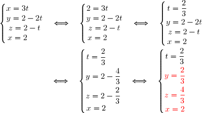
\,.)

\\ \overset{ { \white{ . } } } { M(3\;;\;0\;;\;1)}\end{matrix}\right.\quad\Longrightarrow\quad\overset{ { \white{ . } } } { \overrightarrow{ PM }\begin{pmatrix}3-2\\0-\dfrac2 3\\\overset{ { \phantom{ . } } } { 1-\dfrac 4 3 }\end{pmatrix} =\begin{pmatrix}1\\-\dfrac 2 3\\\overset{ { \phantom{ . } } } { -\dfrac 1 3 }\end{pmatrix} } \\ \\ \left\lbrace\begin{matrix}P\left(2\;;\;\dfrac 2 3\;;\;\dfrac 4 3\right)\\ \overset{ { \phantom{ . } } } { N(3\;;\;1\;;\;1)}\end{matrix}\right.\quad\Longrightarrow\quad\overset{ { \white{ . } } } { \overrightarrow{ PN }\begin{pmatrix}3-2\\1-\dfrac2 3\\\overset{ { \phantom{ . } } } { 1-\dfrac 4 3 }\end{pmatrix} =\begin{pmatrix}1\\\dfrac 1 3\\\overset{ { \phantom{ . } } } { -\dfrac 1 3 }\end{pmatrix} } )
 \\ \phantom{\text{D'où }\;\overrightarrow{PM}\cdot\overrightarrow{PN}}=1-\dfrac 2 9 +\dfrac 1 9 \\ \phantom{\text{D'où }\;\overrightarrow{PM}\cdot\overrightarrow{PN}}=\dfrac 8 9 \\ \\ \Longrightarrow \boxed{ \overrightarrow{PM}\cdot\overrightarrow{PN}=\dfrac 8 9 })
^2+\left(-\dfrac 1 3 \right)^2} \\ \overset{ { \white{ . } } } { \phantom{XXXXW}=\sqrt{1+\dfrac 4 9 +\dfrac 1 9 } } \\ \overset{ { \white{ . } } } { \phantom{XXXXW}=\sqrt{\dfrac {14}{ 9 }} } \\ \\ \text{D'où }\quad\boxed{PM=\dfrac{\sqrt{14}}{3}})


 \quad\Longleftrightarrow\quad \dfrac 8 9=\dfrac{\sqrt{14}}{3}\times\dfrac{\sqrt{11}}{3}\times\cos\left(\widehat{MPN}\right) \\ \overset{ { \white{ . } } } { \phantom{WWWWWWWWWWWWWWWW} \quad\Longleftrightarrow\quad \dfrac 8 9=\dfrac{\sqrt{154}}{9}\times\cos\left(\widehat{MPN}\right) } \\ \overset{ { \white{ . } } } { \phantom{WWWWWWWWWWWWWWWW} \quad\Longleftrightarrow\quad 8=\sqrt{154}\times\cos\left(\widehat{MPN}\right) } \\ \overset{ { \white{ . } } } { \phantom{WWWWWWWWWWWWWWWW} \quad\Longleftrightarrow\quad \cos\left(\widehat{MPN}\right) =\dfrac{8}{\sqrt{154}} } \\\\\text{D'où }\;\boxed{ \widehat{MPN}\approx49,86^{\circ} })
 ne dépasse pas 55°.
 .
.\\ \overset{ { \white{ . } } } { N(3\;;\;1\;;\;1)}\end{matrix}\right.\quad\Longrightarrow\quad\overset{ { \white{ . } } } { \overrightarrow{ EN }\begin{pmatrix}3-0\\1-0\\1-2\end{pmatrix} =\begin{pmatrix}3\\1\\-1\end{pmatrix} })

. })
 } }\times s \end{array}\ \ \ (s\in\mathbb{ R }))
:\left\lbrace\begin{array}l x=3s\\y=s\\z=2-s \end{array}\ \ \ (s\in\mathbb{ R }) } })


\,. })
 }) .
.=\begin{pmatrix}4\\k\end{pmatrix}\times0,6^k\times0,4^{4-k } })
=\begin{pmatrix}4\\0\end{pmatrix}\times0,6^0\times0,4^{4-0 }=1\times1\times0,4^{4 }=0,4^{4 }=0,0256 \\ \overset{ { \white{ . } } } { P(X=1)=\begin{pmatrix}4\\1\end{pmatrix}\times0,6^1\times0,4^{4-1 }=4\times0,6\times0,4^{3 }=0,1536} \\ \overset{ { \white{ . } } } { P(X=2)=\begin{pmatrix}4\\2\end{pmatrix}\times0,6^2\times0,4^{4-2 }=6\times0,6^2\times0,4^{2 }=0,3456} \\ \overset{ { \white{ . } } } { P(X=3)=\begin{pmatrix}4\\3\end{pmatrix}\times0,6^3\times0,4^{4-3 }=4\times0,6^3\times0,4=0,3456} \\ \overset{ { \phantom{ . } } } { P(X=4)=\begin{pmatrix}4\\4\end{pmatrix}\times0,6^4\times0,4^{4-4 }=1\times0,6^4\times1=0,1296})
&&0,0256&&&0,1536& &&0,3456&&&0,3456&&&0,1296&\\&&&&&&&&&&&&&&&\\ \hline \end{array})
 Vérifions si la condition n°1 est vérifiée, soit si
 \ge0,80.)
=p(X=2)+p(X=3)+p(X=4) \\ \overset{ { \white{ . } } } { \phantom{ p(X\ge2) }=0,3456+0,3456+0,1296 } \\ \overset{ { \white{ . } } } { \phantom{ p(X\ge2) }=0,8208 } \\ \\ \Longrightarrow\boxed{ p(X\ge2)\ge0,80 })
}&&&&&&&&&&&&&&&\\ \hline \end{array})
 }) de la variable aléatoire T .
de la variable aléatoire T .=0\times p(T=0)+5\times p(T=5)+9\times p(T=9)+11\times p(T=11))
=p(X\le1)=0,0256+0,1536=0,1792\\\overset{ { \white{ . } } } { p(T=5)=p(X=2)=0,3456\phantom{WWWWWWWW}}\\\overset{ { \white{ . } } } { p(T=9)=p(X=3)=0,3456\phantom{WWWWWWWW}}\\\overset{ { \white{ . } } } { p(T=11)=p(X=4)=0,1296\phantom{WWWWWWWW}}\end{matrix}\right. \\\\\text{Donc }\;E(T)=0\times 0,1792+5\times 0,3456+9\times 0,3456+11\times 0,1296=6,264 \\ \\ \Longrightarrow\boxed{E(T)=6,264})
>6.)
 Voir la correction
 forum de terminale