L'usage de la calculatrice avec mode examen actif est autorisé.
L'usage de la calculatrice sans mémoire, « type collège » est autorisé.
La qualité de la rédaction, la clarté et la précision des raisonnements seront prises en compte dans l'appréciation de la copie.
Les traces de recherche, même incomplètes ou infructueuses seront valorisées.
On considère la fonction g définie sur ]0 ; +[ par
1.Calculons
Il s'ensuit que
Calculons
Il s'ensuit que
2. On admet que la fonction g est dérivable sur ]0 ; +[.
Nous devons étudier les variations de la fonction g sur l'intervalle ]0 ; +[.
Or
Donc
Nous en déduisons que la fonction g est strictement croissante sur ]0 ; +[.
3. a) Montrons qu'il existe un unique réel strictement positif tel que
La fonction g est continue sur l'intervalle ]0 ; +[ car elle est dérivable sur cet intervalle.
La fonction g est strictement croissante sur l'intervalle ]0 ; +[.
Selon le corollaire du théorème des valeurs intermédiaires, il existe un unique réel appartenant à ]0 ; +[ tel que .
3. b)
4. Nous devons dresser le tableau de signe de la fonction g sur l'intervalle ]0 ; +[.
Nous avons montré que la fonction g est strictement croissante sur ]0 ; +[ et que
Nous pouvons alors en déduire le tableau de signe de la fonction g sur l'intervalle ]0 ; +[.
Partie B
On considère la fonction f définie sur l'intervalle ]0 ; +[ par :
1. a) Calculons
1. b) Nous en déduisons que la courbe admet une asymptote verticale d'équation x = 0.
2. Calculons
3. On admet que la fonction f est dérivable sur l'intervalle ]0 ; +[.
Pour tout x ]0 ; +[,
4. Nous déduisons de la question précédente le tableau de variations de la fonction f sur l'intervalle ]0 ; +[.
Par conséquent, la fonction f est strictement décroissante sur ]0 ; ] et est strictement croissante sur [ ; +[.
Partie C
Nous devons étudier la position relative de la courbe et de la courbe représentative de la fonction ln sur l'intervalle ]0 ; +[.
Etudions le signe de la différence sur l'intervalle ]0 ; +[.
Pour tout x ]0 ; +[,
Dès lors, nous obtenons le tableau de signes suivant :
D'où, sur l'intervalle ]0 ; 1[, la courbe est au-dessus de la courbe représentative de la fonction ln, sur l'intervalle ]1 ; +[, la courbe est en dessous de la courbe représentative de la fonction ln, au point (1 ; 0), la courbe traverse la courbe représentative de la fonction ln,
5 points
exercice 2
1. Arbre pondéré représentant la situation pour les 2e et 3e jours.
2. Nous devons calculer , soit
Les événements et forment une partition de l'univers.
En utilisant la formule des probabilités totales, nous obtenons :
3. Nous devons calculer
D'où sachant que le 3e jour, M Durant utilise son vélo, la probabilité qu'il ait pris les transports en commun la veille est égale à
4. Arbre pondéré représentant la situation pour les n-ième et (n +1)-ième jours.
5. Montrons que pour tout entier naturel n non nul,
Les événements et forment une partition de l'univers.
En utilisant la formule des probabilités totales, nous obtenons :
6. Nous devons montrer par récurrence que, pour tout entier naturel n non nul, on a :
Initialisation : Montrons que la propriété est vraie pour n = 1, soit que
C'est une évidence car
Donc l'initialisation est vraie.
Hérédité : Montrons que si pour un nombre naturel n non nul fixé, la propriété est vraie au rang n , alors elle est encore vraie au rang (n +1).
Montrons donc que si pour un nombre naturel n non nul fixé, , alors
En effet,
D'où l'hérédité est vraie.
Puisque l'initialisation et l'hérédité sont vraies, nous avons montré par récurrence que
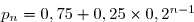
7. Nous devons déterminer la limite de la suite (pn ).
Donc, à très long terme, la probabilité que M. Durand utilise les transports en commun se rapprochera de 0,75.
5 points
exercice 3
1. Une primitive de la fonction f , définie sur par est la fonction F , définie sur par
La fonction F est dérivable sur (produit de deux fonctions dérivables sur ).
Pour tout
Par conséquent, une primitive de la fonction f , définie sur par est la fonction F , définie sur par
Donc la réponse b est correcte.
2. On considère la fonction g définie par
La fonction g est définie sur ]- ; -2[ ]1 ; +[
En effet, la fonction g est définie si
Étudions le signe de
D'où
Par conséquent, la fonction g est définie sur ]- ; -2[ ]1 ; +[.
Donc la réponse c est correcte.
3. La fonction h définie sur par est concave sur ]- ; -3] et convexe sur [-3 ; +[
La concavité de la fonction h se détermine selon le signe de la dérivée seconde h''(x) .
La fonction h est dérivable sur (produit de fonctions dérivables sur ).
Pour tout nombre réel x ,
La fonction dérivée h' est dérivable sur (produit de fonctions dérivables sur ).
Pour tout nombre réel x ,
Étudions le signe de h''(x) sur
Par conséquent, la fonction h est concave sur ]- ; -3] et convexe sur [-3 ; +[.
Donc la réponse d est correcte.
4. Une suite (un ) est minorée par 3 et converge vers un réel On peut affirmer que
La suite (un ) est minorée par 3.
Il s'ensuit que pour tout entier naturel n , un 3.
De plus,
Par conséquent,
Donc la réponse b est correcte.
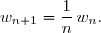
5. La suite (wn ) est définie par et pour tout entier naturel n strictement positif,
La suite (wn ) converge vers 0
Calculons les premiers termes de la suite (wn ).
Nous pouvons conjecturer que la suite (wn ) converge vers 0.
Démontrons cette conjecture.
Démontrons d'abord par récurrence que pour tout entier naturel n strictement positif,
Initialisation : Montrons que la propriété est vraie pour n = 1, soit que
C'est une évidence car
Donc l'initialisation est vraie.
Hérédité : Montrons que si pour un nombre naturel non nul n fixé, la propriété est vraie au rang n , alors elle est encore vraie au rang (n +1).
Montrons donc que si pour un nombre naturel non nul n fixé, , alors
En effet,
L'hérédité est vraie.
Puisque l'initialisation et l'hérédité sont vraies, nous avons montré par récurrence que
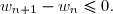
Démontrons ensuite que la suite (wn ) est décroissante.
Pour tout entier naturel n strictement positif,
Or
D'où
Nous en déduisons que la suite (wn ) est décroissante.
En conséquence, la suite (wn ) est décroissante et minorée par 0.
Elle converge alors vers sa borne inférieure.
Dès lors, la suite (wn ) converge vers 0.
Donc la réponse d est correcte.
5 points
exercice 4
Dans l'espace muni d'un repère orthonormée
on considère les points A (-1 ; -3 ; 2), B (3 ; -2 ; 6) et C (1 ; 2 ; -4).
1. Nous montrerons que les points A , B et C définissent un plan en montrant qu'ils ne sont pas colinéaires.
Montrons donc que les vecteurs et ne sont pas colinéaires.
Nous avons : A (-1 ; -3 ; 2), B (3 ; -2 ; 6) et C (1 ; 2 ; -4).
Dès lors,
Les vecteurs et ne sont manifestement pas colinéaires.
D'où les points A , B et C ne sont pas alignés.
Par conséquent, les points A , B et C définissent un plan noté .
2. a) Montrons que le vecteur est normal au plan .
Le vecteur est orthogonal à deux vecteurs et non colinéaires du plan .
Donc le vecteur est un vecteur normal au plan .
2. b) Déterminons une équation du plan .
Nous savons que tout plan de vecteur normal admet une équation cartésienne de la forme : ax + by + cz + d = 0.
Puisque le vecteur est normal au plan , nous déduisons qu'une équation cartésienne du plan est de la forme : 13x - 16y - 9z + d = 0.
Or le point A (-1 ; -3 ; 2) appartient au plan . Ses coordonnées vérifient l'équation du plan.
D'où 13(-1) - 16(-3) - 92 + d = 0 , soit d = -17.
Par conséquent, une équation cartésienne du plan est
On note la droite passant par le point F (15 ; -16 ; -8) et orthogonale à .
3. Nous devons donner une représentation paramétrique de la droite .
Puisque la droite est orthogonale au plan , le vecteur est un vecteur directeur de la droite .
La droite passe par le point
D'où une représentation paramétrique de la droite est donnée par :
soit
4. On appelle E le point d'intersection de la droite et du plan . Déterminons les coordonnées du point E .
Le point E appartient à .
Donc les coordonnées de E sont de la forme
Le point E appartient au plan .
Donc ses coordonnées vérifient l'équation de
Nous obtenons ainsi :
Remplaçons t par (-1) dans les coordonnées de E .
Par conséquent, le point E a pour coordonnées
5. Nous devons calculer la distance du point F au plan .
Cette distance est donnée par FE.
Par conséquent, la distance du point F au plan est égale à
6. Nous devons déterminer les coordonnées du ou des point(s) de la droite dont la distance au plan est égale à la moitié de la distance du point F au plan .
Soit M un point quelconque de la droite .
Les coordonnées de M sont de la forme .
La distance du point M au plan est donnée par ME.
Par conséquent, la distance du point M au plan est
La distance du point F au plan est donnée par (voir question 5.)
Nous devons déterminer les coordonnées de M vérifiant la condition
Par conséquent, les deux points de la droite dont la distance au plan est égale à la moitié de la distance du point F au plan ont pour coordonnées et
Publié par malou
le
ceci n'est qu'un extrait
Pour visualiser la totalité des cours vous devez vous inscrire / connecter (GRATUIT) Inscription Gratuitese connecter
Merci à Hiphigenie / malou pour avoir contribué à l'élaboration de cette fiche
Désolé, votre version d'Internet Explorer est plus que périmée ! Merci de le mettre à jour ou de télécharger Firefox ou Google Chrome pour utiliser le site. Votre ordinateur vous remerciera !
 [ par
[ par =\ln(x^2)+x-2.)
 Calculons
 . })
=-\infty\phantom{ W } }\end{matrix}\right.\quad\underset{ (X=x^2) }{ \Longrightarrow }\quad\lim\limits_{ x\to0^+ }\ln\,(x^2)=-\infty \\ \phantom{ WWWWWWvWWWW }\Longrightarrow\quad\quad\lim\limits_{ x\to0^+ }(\ln\,(x^2)+x)=-\infty \\ \\ \phantom{ WWWWWWvWWWW }\Longrightarrow\quad\quad\lim\limits_{ x\to0^+ }(\ln\,(x^2)+x-2)=-\infty)
=-\infty }. } )
. })
=+\infty\phantom{ W } }\end{matrix}\right.\quad\underset{ (X=x^2) }{ \Longrightarrow }\quad\lim\limits_{ x\to+\infty }\ln\,(x^2)=+\infty \\ \phantom{ WWWWWWvWWWW }\Longrightarrow\quad\quad\lim\limits_{ x\to+\infty }(\ln\,(x^2)+x)=+\infty \\ \\ \phantom{ WWWWWWvWWWW }\Longrightarrow\quad\quad\lim\limits_{ x\to+\infty }(\ln\,(x^2)+x-2)=+\infty)
=+\infty }. } )

![\forall\,x\in\;]0\;;\;+\infty\,[,\;g'(x)=[\ln(x^2)+x-2]' \\ \overset{ { \white{ . } } } { \phantom{\forall\,x\in\;]0\;;\;+\infty\,[,\;g'(x)}=\dfrac{(x^2)'}{x^2}+1} \\ \overset{ { \white{ . } } } { \phantom{\forall\,x\in\;]0\;;\;+\infty\,[,\;g'(x)}=\dfrac{2x}{x^2}+1} \\ \overset{ { \white{ . } } } { \phantom{\forall\,x\in\;]0\;;\;+\infty\,[,\;g'(x)}=\dfrac{2}{x}+1} \\ \\ \Longrightarrow\quad\boxed{\forall\,x\in\;]0\;;\;+\infty\,[,\;g'(x)=\dfrac{2}{x}+1}](https://latex.ilemaths.net/latex-0.tex?\forall\,x\in\;]0\;;\;+\infty\,[,\;g'(x)=[\ln(x^2)+x-2]' \\ \overset{ { \white{ . } } } { \phantom{\forall\,x\in\;]0\;;\;+\infty\,[,\;g'(x)}=\dfrac{(x^2)'}{x^2}+1} \\ \overset{ { \white{ . } } } { \phantom{\forall\,x\in\;]0\;;\;+\infty\,[,\;g'(x)}=\dfrac{2x}{x^2}+1} \\ \overset{ { \white{ . } } } { \phantom{\forall\,x\in\;]0\;;\;+\infty\,[,\;g'(x)}=\dfrac{2}{x}+1} \\ \\ \Longrightarrow\quad\boxed{\forall\,x\in\;]0\;;\;+\infty\,[,\;g'(x)=\dfrac{2}{x}+1} )
![x\in\;]0\;;\;+\infty\,[\quad\Longrightarrow\dfrac{2}{x}+1>0](https://latex.ilemaths.net/latex-0.tex?x\in\;]0\;;\;+\infty\,[\quad\Longrightarrow\dfrac{2}{x}+1>0)
![\boxed{\forall\,x\in\;]0\;;\;+\infty\,[,\;g'(x)>0}](https://latex.ilemaths.net/latex-0.tex?\boxed{\forall\,x\in\;]0\;;\;+\infty\,[,\;g'(x)>0})
 tel que
 =0\,. })
![\left\lbrace\begin{matrix}\lim\limits_{ x\to0^+ }g(x)=-\infty\phantom{ ww }\\\lim\limits_{ x\to+\infty }g(x)=+\infty\phantom{ ww } \end{matrix}\right.\quad\Longrightarrow\quad \boxed{ 0\in\,]\,\lim\limits_{ x\to0^+ }g(x)\,;\,\lim\limits_{ x\to+\infty }g(x)\,[ }](https://latex.ilemaths.net/latex-0.tex?\left\lbrace\begin{matrix}\lim\limits_{ x\to0^+ }g(x)=-\infty\phantom{ ww }\\\lim\limits_{ x\to+\infty }g(x)=+\infty\phantom{ ww } \end{matrix}\right.\quad\Longrightarrow\quad \boxed{ 0\in\,]\,\lim\limits_{ x\to0^+ }g(x)\,;\,\lim\limits_{ x\to+\infty }g(x)\,[ })
\approx-0,00038<0\\g(1,38)\approx0,024>0\phantom{xxx}\end{matrix}\right.\quad\Longrightarrow\quad\boxed{ 1,37<\alpha<1,38 }\,.)
&||&-&&0&&+&\\&||&&& &&&\\ \hline \end{array})
=\dfrac{x-2}{x}\,\ln(x)\,.)
. })
=-2 \\ \overset{ { \white{ . } } }{ \lim\limits_{ x\to0^+ }x=0^+\phantom{ Ww } }\\ \overset{ { \white{ . } } }{ \lim\limits_{ x\to0^+ }\ln(x)=-\infty\phantom{ } }\end{matrix}\right.\quad\Longrightarrow \quad \left\lbrace\begin{matrix}\lim\limits_{ x\to0^+ }\dfrac{x-2}{x}=-\infty \\\overset{ { \white{ . } } }{ \lim\limits_{ x\to0^+ }\ln(x)=-\infty\phantom{ } }\end{matrix}\right. \quad\Longrightarrow \quad\lim\limits_{ x\to0^+ }\dfrac{x-2}{x}\,\ln(x)=+\infty\\ \\ \\ \quad\Longrightarrow\quad\boxed{\lim\limits_{ x\to0^+ }f(x)=+\infty})
 admet une asymptote verticale d'équation x = 0.
. })
![\forall\,x\in\,]\,0\;;\;+\infty\,[,\;f(x)=\dfrac{x-2}{x}\,\ln(x)=\left(\dfrac x x -\dfrac 2 x\right)\ln(x) \\ \\ \quad\Longrightarrow\quad \boxed{ \forall\,x\in\,]\,0\;;\;+\infty\,[,\;f(x)=\left(1 -\dfrac 2 x\right)\ln(x)} \\ \\ \text{Or }\;\left\lbrace\begin{matrix}\lim\limits_{x\to+\infty }\left(1 -\dfrac 2 x\right)=1-0=1 \\ \overset{ { \white{ . } } }{ \lim\limits_{ x\to+\infty }\ln(x)=+\infty\phantom{ Ww } }\end{matrix}\right.\quad\Longrightarrow\quad \lim\limits_{x\to+\infty }\left(1 -\dfrac 2 x\right)\ln(x)=+\infty \\ \\ \\ \Longrightarrow\quad\boxed{ \lim\limits_{x\to+\infty }f(x)=+\infty }\,.](https://latex.ilemaths.net/latex-0.tex?\forall\,x\in\,]\,0\;;\;+\infty\,[,\;f(x)=\dfrac{x-2}{x}\,\ln(x)=\left(\dfrac x x -\dfrac 2 x\right)\ln(x) \\ \\ \quad\Longrightarrow\quad \boxed{ \forall\,x\in\,]\,0\;;\;+\infty\,[,\;f(x)=\left(1 -\dfrac 2 x\right)\ln(x)} \\ \\ \text{Or }\;\left\lbrace\begin{matrix}\lim\limits_{x\to+\infty }\left(1 -\dfrac 2 x\right)=1-0=1 \\ \overset{ { \white{ . } } }{ \lim\limits_{ x\to+\infty }\ln(x)=+\infty\phantom{ Ww } }\end{matrix}\right.\quad\Longrightarrow\quad \lim\limits_{x\to+\infty }\left(1 -\dfrac 2 x\right)\ln(x)=+\infty \\ \\ \\ \Longrightarrow\quad\boxed{ \lim\limits_{x\to+\infty }f(x)=+\infty }\,.)
 ]0 ; +
![f'(x)=\left[\dfrac{x-2}{x}\,\ln(x)\right]' \\ \phantom{f'(x)}=\left(\dfrac{x-2}{x}\right)'\times\ln(x)+\dfrac{x-2}{x}\times [\ln (x)]' \\ \overset{ { \phantom{ . } } } {\phantom{f'(x)}=\dfrac{(x-2)'\times x-(x-2)\times x'}{x^2}\times\ln (x)+\dfrac{x-2}{x}\times \dfrac 1 x } \\ \overset{ { \phantom{ . } } } {\phantom{f'(x)}=\dfrac{1\times x-(x-2)\times 1}{x^2}\times\ln (x)+\dfrac{x-2}{x^2} } \\ \overset{ { \phantom{ . } } } {\phantom{f'(x)}=\dfrac{ x-x+2}{x^2}\times\ln (x)+\dfrac{x-2}{x^2} }](https://latex.ilemaths.net/latex-0.tex?f'(x)=\left[\dfrac{x-2}{x}\,\ln(x)\right]' \\ \phantom{f'(x)}=\left(\dfrac{x-2}{x}\right)'\times\ln(x)+\dfrac{x-2}{x}\times [\ln (x)]' \\ \overset{ { \phantom{ . } } } {\phantom{f'(x)}=\dfrac{(x-2)'\times x-(x-2)\times x'}{x^2}\times\ln (x)+\dfrac{x-2}{x}\times \dfrac 1 x } \\ \overset{ { \phantom{ . } } } {\phantom{f'(x)}=\dfrac{1\times x-(x-2)\times 1}{x^2}\times\ln (x)+\dfrac{x-2}{x^2} } \\ \overset{ { \phantom{ . } } } {\phantom{f'(x)}=\dfrac{ x-x+2}{x^2}\times\ln (x)+\dfrac{x-2}{x^2} })
![\\ \overset{ { \phantom{ . } } } {\phantom{f'(x)}=\dfrac{2}{x^2}\times\ln (x)+\dfrac{x-2}{x^2} } \\ \overset{ { \phantom{ p } } } {\phantom{f'(x)}=\dfrac{2\ln(x)}{x^2}+\dfrac{x-2}{x^2} } \\ \overset{ { \phantom{ p } } } {\phantom{f'(x)}=\dfrac{\ln(x^2)+x-2}{x^2} } \\ \overset{ { \phantom{ p } } } {\phantom{f'(x)}=\dfrac{g(x)}{x^2} } \\\\ \Longrightarrow\quad \boxed{ \forall\,x\,\in,]\,0\;;\;+\infty\,[,\;f'(x)=\dfrac{g(x)}{x^2} }](https://latex.ilemaths.net/latex-0.tex?\\ \overset{ { \phantom{ . } } } {\phantom{f'(x)}=\dfrac{2}{x^2}\times\ln (x)+\dfrac{x-2}{x^2} } \\ \overset{ { \phantom{ p } } } {\phantom{f'(x)}=\dfrac{2\ln(x)}{x^2}+\dfrac{x-2}{x^2} } \\ \overset{ { \phantom{ p } } } {\phantom{f'(x)}=\dfrac{\ln(x^2)+x-2}{x^2} } \\ \overset{ { \phantom{ p } } } {\phantom{f'(x)}=\dfrac{g(x)}{x^2} } \\\\ \Longrightarrow\quad \boxed{ \forall\,x\,\in,]\,0\;;\;+\infty\,[,\;f'(x)=\dfrac{g(x)}{x^2} })
&||&-&&0&&+&\\x^2&0&+&&+&&+&\\&||&&& &&&\\ \hline&||&&&&&&\\\ f'(x)&||&-&&0&&+&\\&||&&& &&&\\ \hline&+\infty&&&&&&+\infty\\\ f(x)&||&\searrow&&&&\nearrow&\\&||&&&f(\alpha) &&&\\ \hline \end{array})
 est strictement croissante sur [
-\ln(x) }) sur l'intervalle ]0 ; +
sur l'intervalle ]0 ; +-\ln(x)=\dfrac{x-2}{x}\,\ln(x)-\ln(x) \\ \overset{ { \white{ . } } } { \phantom{f(x )-\ln(x) }= \left(\dfrac{x-2}{x}-1\right)\ln(x) } \\ \overset{ { \white{ . } } } { \phantom{f(x )-\ln(x) }= \dfrac{x-2-x}{x}\,\ln(x) } \\ \overset{ { \white{ . } } } { \phantom{f(x )-\ln(x) }= \dfrac{-2}{x}\,\ln(x) } \\ \\ \Longrightarrow\quad\boxed{f(x)-\ln(x)= \dfrac{-2\,\ln(x)}{x} } )
=0\Longleftrightarrow x=1\\ \ln (x)>0\Longleftrightarrow x>1\\ \phantom{xxi}\ln (x)<0\Longleftrightarrow 0<x<1\end{matrix}\phantom{ WW } \begin{matrix}|\\|\\|\\|\\|\\|\\|\\|\\|\end{matrix}\phantom{ WW }\begin{array} { |c|ccccccc| } \hline &&&&&&&& x &0&&&1&&&+\infty\\ &&&&&&& \\ \hline&&&&&&& \\-2&&-&&-&&-&\\ \ln (x)&||& - && 0 & &+ &\\ \ x&0& + && + & &+ &\\&&&&&&&\\ \hline&||&&&&&&\\ \dfrac{-2\,\ln(x)}{x}&||&+&&0&&-&\\&||&&& &&&\\ \hline \end{array})
 sur l'intervalle ]1 ; +
 , soit
 \,.})
 et
et  forment une partition de l'univers.
=p(T_2\cap T_3)+p(V_2\cap T_3) \\ \overset{ { \white{ . } } }{ \phantom{ p(T_3) }=p(T_2)\times p_{ T_2 }(T_3)+p(V_2)\times p_{ V_2 }(T_3)} \\ \overset{ { \white{ . } } }{ \phantom{ p(T_3) }=0,8\times0,8+0,2\times0,6 } \\ \overset{ { \white{ . } } }{ \phantom{ p(T_3) }=0,64+0,12 })
 }=0,76 } \\ \\ \Longrightarrow\quad\boxed{ p_3=p(T_3)=0,76 }\,.)
\,. })
=\dfrac{ p(T_2\cap V_3) } { p(V_3) } \\ \overset{ { \white{ . } } } { \phantom{ p_{V_3}(T_2) } =\dfrac{ p(T_2)\times p_{T_2}(V_3) } { 1-p(T_3) } } \\ \overset{ { \white{ . } } } { \phantom{ p_{V_3}(T_2) } =\dfrac{ 0,8\times0,2 } { 1-0,76} } \\ \overset{ { \white{ . } } } { \phantom{ p_{V_3}(T_2) } =\dfrac{ 0,16 }{ 0,24 } =\dfrac{16 } { 24 } } \\ \overset{ { \phantom{ . } } } { \phantom{ p_{V_3}(T_2) } =\dfrac{2 } { 3 } } \\ \\ \Longrightarrow\boxed{ p_{V_3}(T_2)=\dfrac{ 2}{ 3 } } )

 et
et  forment une partition de l'univers.
=p(T_n\cap T_{n+1})+p(V_n\cap T_{n+1}) \\ \overset{ { \white{ . } } }{ \phantom{ p_{n+1}=p(T_{n+1}) }=p(T_n)\times p_{ T_n }(T_{n+1})+p(V_n)\times p_{ V_n }(T_{n+1})} \\ \overset{ { \white{ . } } }{ \phantom{ p_{n+1}=p(T_{n+1}) }=p_n\times0,8+(1-p_n)\times0,6 } \\ \overset{ { \white{ . } } }{ \phantom{ p_{n+1}=p(T_{n+1}) }=0,8p_n+0,6-0,6p_n } )
 }=0,2p_n+0,6. } \\ \\ \Longrightarrow\quad\boxed{ p_{n+1}=0,2p_n+0,6 }\,.)


 , alors
+0,6 } \\ \overset{ { \white{ . } } } { \phantom{\forall\,n\in\N^*,\; p_{n+1} }=0,2\times0,75+0,25\times 0,2\times 0,2^{n-1}+0,6 } \\ \overset{ { \white{ . } } } { \phantom{\forall\,n\in\N^*,\; p_{n+1} }=0,15+0,25\times 0,2^{n}+0,6 })


=0,75 } \\\\ \Longrightarrow\quad\boxed{\lim\limits_{n\to +\infty}p_n=0,75 })
 par
par =x\,\text{e}^x\,, }) est la fonction F , définie sur
est la fonction F , définie sur  par
par =(x-1)\,\text e^x}\quad {\red{\longrightarrow\quad\text{Réponse b.}}})

=(x-1)'\times\text e^x+(x-1)\times(\text e^x)' \\ \overset{ { \white{ . } } } { \phantom{F\,'(x)}=1\times\text e^x+(x-1)\times \text e^x } \\ \overset{ { \white{ . } } } { \phantom{F\,'(x)}=(1+x-1)\, \text e^x } \\ \overset{ { \white{ . } } } { \phantom{F\,'(x)}=x\, \text e^x })
}=f(x)} \\ \\ \Longrightarrow\quad \boxed{ \forall\,x\in\R, F\,'(x)=f(x)})
=(x-1)\,\text e^x }.)
=\ln\left(\dfrac{ x-1 } { 2x+4 }\right).)
 ]1 ; +


![\overset{ { \white{ . } } } { \dfrac{ x-1 } { 2x+4 }>0\quad\Longleftrightarrow\quad x\in\,]-\infty\;;\;-2[\;\cup\;]1\;;\;+\infty\,[. }](https://latex.ilemaths.net/latex-0.tex?\overset{ { \white{ . } } } { \dfrac{ x-1 } { 2x+4 }>0\quad\Longleftrightarrow\quad x\in\,]-\infty\;;\;-2[\;\cup\;]1\;;\;+\infty\,[. })
=(x+1)\text e^x }) est concave sur ]-
est concave sur ]-
=(x+1)'\times\text e^x+(x+1)\times(\text e^x)' \\ \overset{ { \white{ . } } } { \phantom{h'(x)}=1\times\text e^x+(x+1)\times\text e^x } \\ \overset{ { \white{ . } } } { \phantom{h'(x)}=(1+x+1)\,\text e^x } \\ \overset{ { \white{ . } } } { \phantom{h'(x)}=(x+2)\,\text e^x } \\ \\ \Longrightarrow\quad\boxed{\forall\,x\in\R,\;h'(x)=(x+2)\,\text e^x })
=(x+2)'\times\text e^x+(x+2)\times(\text e^x)' \\ \overset{ { \white{ . } } } { \phantom{h''(x)}=1\times\text e^x+(x+2)\times\text e^x } \\ \overset{ { \white{ . } } } { \phantom{h''(x)}=(1+x+2)\,\text e^x } \\ \overset{ { \white{ . } } } { \phantom{h''(x)}=(x+3)\,\text e^x } \\ \\ \Longrightarrow\quad\boxed{\forall\,x\in\R,\;h''(x)=(x+3)\,\text e^x })

![\begin{matrix}x+3=0\Longleftrightarrow x=-3\\ x+3>0\Longleftrightarrow x>-3\\ x+3<0\Longleftrightarrow x<-3\end{matrix}\phantom{ WW } \begin{matrix}|\\|\\|\\|\\|\\|\\|\\|\\|\end{matrix}\phantom{ WW }\begin{array} { |c|ccccccc| } \hline &&&&&&&& x &-\infty&&&-3&&&+\infty\\ &&&&&&& \\ \hline&&&&&&&\\ x+3&& - && 0&&+& \\ \text e^x&& + && + & &+ &\\&&&&&&&\\ \hline&&&&&&&\\ f''(x)=(x+3)\text e^x&& -&&0 & &+ &\\&&&&&&&\\ \hline \end{array} \\\\\text{D'où }\;f''(x)\le0\quad\Longleftrightarrow\quad x\in\,]-\infty\;;\;-3\,] \\\overset{ { \white{ . } } } { \phantom{\text{D'où }}\;f''(x)\ge0\quad\Longleftrightarrow\quad x\in\,[-3\;;\;+\infty[ }](https://latex.ilemaths.net/latex-0.tex?\begin{matrix}x+3=0\Longleftrightarrow x=-3\\ x+3>0\Longleftrightarrow x>-3\\ x+3<0\Longleftrightarrow x<-3\end{matrix}\phantom{ WW } \begin{matrix}|\\|\\|\\|\\|\\|\\|\\|\\|\end{matrix}\phantom{ WW }\begin{array} { |c|ccccccc| } \hline &&&&&&&& x &-\infty&&&-3&&&+\infty\\ &&&&&&& \\ \hline&&&&&&&\\ x+3&& - && 0&&+& \\ \text e^x&& + && + & &+ &\\&&&&&&&\\ \hline&&&&&&&\\ f''(x)=(x+3)\text e^x&& -&&0 & &+ &\\&&&&&&&\\ \hline \end{array} \\\\\text{D'où }\;f''(x)\le0\quad\Longleftrightarrow\quad x\in\,]-\infty\;;\;-3\,] \\\overset{ { \white{ . } } } { \phantom{\text{D'où }}\;f''(x)\ge0\quad\Longleftrightarrow\quad x\in\,[-3\;;\;+\infty[ })


 3.
3.

 et pour tout entier naturel n strictement positif,


 Démontrons d'abord par récurrence que pour tout entier naturel n strictement positif,


 , alors
\phantom{xx}\\ \\w_n\ge0\quad(\text{par hypothèse)}\end{matrix}\right.\quad\Longrightarrow \quad \dfrac 1 n\,w_n\ge0 \quad\Longrightarrow \quad \boxed{ w_{n+1}\ge0}\,.)


\,w_n } \\ \overset{ { \white{ . } } } { \phantom{w_{n+1}-w_n}=\dfrac{1-n}{n}\,w_n })
\\\overset{ { \white{ . } } } { n>0\quad\text{(car }n\in\N^*)\phantom{iW} }\\ \overset{ { \phantom{ . } } } { w_n\ge0\phantom{WWWWWWW}}\end{matrix}\right. \quad\Longrightarrow\quad \boxed{\dfrac{1-n}{n}\,w_n\le0 })
,)
 et
et  ne sont pas colinéaires.
\\-2-(-3)\\6-2\end{pmatrix} =\begin{pmatrix}4\\1\\4\end{pmatrix}\\ \\ \overrightarrow{ AC }\ \begin{pmatrix}1-(-1)\\2-(-3)\\-4-2\end{pmatrix}=\begin{pmatrix}2\\5\\-6\end{pmatrix}\end{matrix}\right. })
 .
. est normal au plan
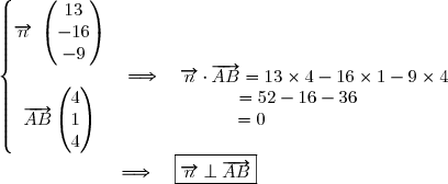
\\=26-80+54\phantom{ wW }\\=0\phantom{ WWWwWwW }\end{matrix} \\ \phantom{ WWWWWW }\Longrightarrow\quad\boxed{ \overrightarrow{ n }\perp\overrightarrow{ AC } })
 est orthogonal à deux vecteurs
  admet une équation cartésienne de la
  (-1) - 16
 la droite passant par le point F (15 ; -16 ; -8) et orthogonale à
  est un vecteur directeur de la droite
 . })
 } }\times t\\z={ \blue{ -8 } }+{ \red{ (-9) } }\times t \end{array}\ \ \ (t\in\mathbb{ R }))
 } })
 Le point E appartient à
 . })
 .
.
-16(-16-16t)-9(-8-9t)-17=0 \\ \overset{ { \white{ . } } } { \phantom{ 4(-1+4t)}\quad\Longleftrightarrow\quad 195+169t+256+256t+72+81t-17=0} \\ \overset{ { \white{ . } } } { \phantom{ 4(-1+4t) }\quad\Longleftrightarrow\quad 506t+506=0 } \\ \overset{ { \white{ . } } } { \phantom{ 4(-1+4t) }\quad\Longleftrightarrow\quad 506t=-506 } \\ \overset{ { \phantom{ . } } } { }\phantom{ 4(-1+4t) }\quad\Longleftrightarrow\quad t=-1)
=(15-13\,;\,-16+16\,;\,-8+9) \\ \overset{ { \white{ . } } } { \phantom{(15+13t\,;\,-16-16t\,;\,-8-9t)}=(2\,;\,0\,;\,1) })
\,.)
 } \\ \overset{ { \white{ . } } }{ 1-(-8) }\end{pmatrix}=\begin{pmatrix}-13\\ 16\\ 9\end{pmatrix} \\ \\ \\ \Longrightarrow\quad FE=\sqrt{ (-13)^2+16^2+9^2} \\ \overset{ { \phantom{ . } } }{ \phantom{ WWWW }=\sqrt{ 169+256+81}} \\ \overset{ { \phantom{ . } } }{ \phantom{ WWWW }=\sqrt{ 506} })

. }) .
.\\ \overset{ { \white{ . } } }{ 0-(-16-16t) } \\ \overset{ { \white{ . } } }{ 1-(-8-9t) }\end{pmatrix}=\begin{pmatrix}-13-13t\\ 16+16t\\ 9+9t\end{pmatrix}\quad\Longrightarrow\quad \overrightarrow{ ME }\ \begin{pmatrix}-13(1+t)\\ \overset{ { \white{ . } } }{ 16(1+t) } \\ \overset{ { \phantom{ . } } }{ 9(1+t) }\end{pmatrix} \\ \\ \\ \Longrightarrow\quad ME=\sqrt{(-13)^2(1+t)^2+16^2(1+t)^2+9^2(1+t)^2} \\ \overset{ { \phantom{ . } } }{ \phantom{ WWWW }=\sqrt{169(1+t)^2+256(1+t)^2+81(1+t)^2}} \\ \overset{ { \phantom{ . } } }{ \phantom{ WWWW }=\sqrt{ 506(1+t)^2} })
^2}.)
 (voir question 5.)

^2}=\dfrac{\sqrt{ 506}}{2} \\ \overset{ { \white{ . } } } {\phantom{WWWWx} \quad\Longleftrightarrow\quad 506(1+t)^2=\dfrac{506}{4}} \\ \overset{ { \white{ . } } } {\phantom{WWWWx} \quad\Longleftrightarrow\quad (1+t)^2=\dfrac{1}{4}} \\ \overset{ { \white{ . } } } {\phantom{WWWWx} \quad\Longleftrightarrow\quad 1+t=\dfrac{1}{2}\quad\text{ou}\quad1+t=-\dfrac{1}{2}} \\ \overset{ { \phantom{ . } } } {\phantom{WWWWx} \quad\Longleftrightarrow\quad t=\dfrac{1}{2}-1\quad\text{ou}\quad t=-\dfrac{1}{2}-1} \\ \overset{ { \phantom{ . } } } {\phantom{WWWWx} \quad\Longleftrightarrow\quad \boxed{t=-\dfrac{1}{2}\quad\text{ou}\quad t=-\dfrac{3}{2}}})
=\dfrac{17}{2}\\\overset{ { \white{ . } } } { y_M=-16-16\times (-\dfrac{1}{2})= -8 } \\\overset{ { \white{ . } } } { z_M=-8-9\times (-\dfrac{1}{2})= -\dfrac{7}{2} }\end{matrix}\right. \\ \\ \quad\Longrightarrow M\left(-\dfrac{17}{2}\;;\;-8\;;\;-\dfrac{7}{2}\right))
=-\dfrac{9}{2}\\\overset{ { \white{ . } } } { y_M=-16-16\times (-\dfrac{3}{2})= 8 } \\\overset{ { \white{ . } } } { z_M=-8-9\times (-\dfrac{3}{2})= \dfrac{11}{2} }\end{matrix}\right. \\ \\ \quad\Longrightarrow M\left(-\dfrac{9}{2}\;;\;8\;;\;\dfrac{11}{2}\right))
 }) et
et \,. })
 Voir la correction
 forum de terminale