Le plan est rapporté à un repère orthonormé direct
Soit A , B et C les points du plan d'affixes respectives et
A tout point M du plan d'affixe on associe le point M' de
d'affixe
1. Nous devons montrer que pour tout
Nous savons que pour tout
Dès lors, pour tout
2. Pour tout
Soit M le point d'affixe z et M' le point d'affixe z' .
3. Nous devons déterminer l'ensemble des points tels que
D'où l'ensemble des points tels que est
4. a) Nous devons montrer que les points A , M et M' sont alignés si et seulement si
Nous avons montré dans la question 2. que
Ainsi, A , M et M' sont alignés
Par conséquent, les points A , M et M' sont alignés si et seulement si
4. b) Nous devons en déduire l'ensemble des points M tels que les points A , M et M' soient alignés.
Les points A , M et M' sont alignés
Par conséquent, l'ensemble des points M tels que les points A , M et M' soient alignés est la réunion des droites (OA ) et (AB ) privée du point A (car ).
5. Nous devons montrer que pour tout point M d'affixe et
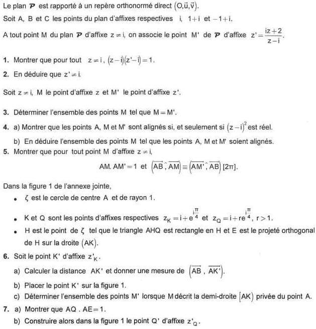
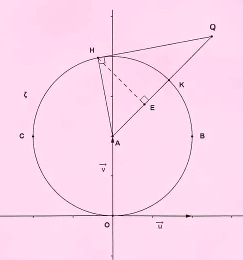
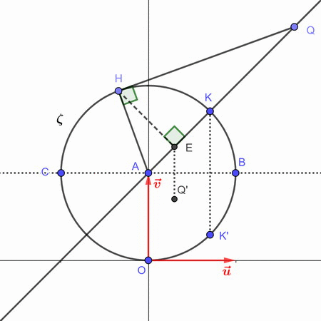
Dans la figure ci-dessous,
est le cercle de centre A et de rayon 1. K et Q sont les points d'affixes respectives et H est le point de tel que le triangle AHQ est rectangle en H et E est le projeté orthogonal de H sur la droite (AK ).
6. Soit le point K' d'affixe .
6. a) Nous devons calculer le distance AK' et donner une mesure de .
Puisque nous savons par la question 5 que et
D'où
6. b) Le point K' appartient au cercle car AK' = 1.
Ce point K' est le symétrique du point K par rapport à la droite (AB ) (voir figure ci-dessus).
6. c) Nous dévons déterminer l'ensemble des points M' lorsque M décrit la demi-droite [AK ) privée du point A .
Soit le point M appartenant à la demi-droite [AK ) privée du point A .
Si z est l'affixe du point M , alors
Dans ce cas,
Puisque nous savons par la question 5 que
Dès lors,
Nous en déduisons que M' appartient à la demi-droite [AK' ) privée du point A .
Par conséquent, l'ensemble des points M' lorsque M décrit la demi-droite [AK ) privée du point A est la demi-droite [AK' ) privée du point A .
7. a) Nous devons montrer que
Le triangle AHQ est rectangle en H .
Le point E est le projeté orthogonal de H sur la droite (AQ).
Le point H est le projeté orthogonal de Q sur la droite (AH ).
Par conséquent,
D'où
7. b) Construisons le point Q' d'affixe
D'une part, nous savons par la question 5 que et par la question 7. a) que
D'où
D'autre part, en utilisant la question 6 a), nous obtenons :
Par conséquent, le point Q' est le symétrique du point E par rapport à la droite (AB ) (voir figure ci-dessus) .
6 points
exercice 2
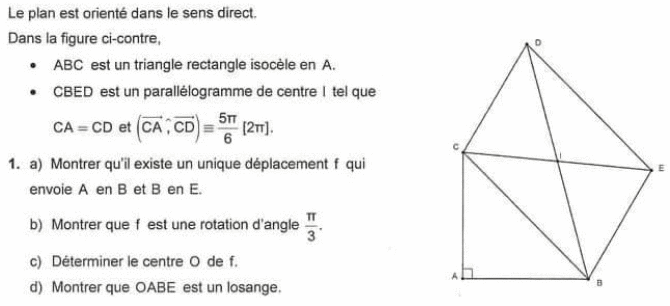
Le plan est orienté dans le sens direct.
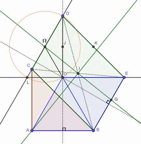
Dans la figure ci-dessous, ABC est un triangle rectangle isocèle en A . CBED est un parallélogramme de centre I tel que et
1. a) Nous devons montrer qu'il existe un unique déplacement f qui envoie A en B et B en E .
Montrons donc que et que
D'une part, car ABC est un triangle.
D'autre part, montrons que
Puisque ABC est un triangle isocèle en A , nous savons que
Selon l'énoncé, nous savons que
Or CBED est un parallélogramme et par suite,
Dès lors,
Nous en déduisons qu'il existe un unique déplacement f qui envoie A en B et B en E .
1. b) Montrons que f est une rotation d'angle
Le déplacement f envoie A en B et B en E .
Donc l'angle du déplacement f est
Dès lors, f est un déplacement d'angle f est un déplacement d'angle non nul et n'est donc pas une translation.
Par conséquent, f est une rotation d'angle
1. c) Déterminons le centre O de f .
Nous savons que et que Le centre O de f est l'intersection des médiatrices des segments [AB ] et [BE ].
1. d) Nous devons montrer que OABE est un losange.
Il s'ensuit que le triangle OAB est équilatéral et que
Il s'ensuit que le triangle OBE est équilatéral et que
D'où
Par conséquent, OABE est un losange.
On note J le milieu du segment [OD ] et on désigne par S la similitude directe qui envoie A en I et O et J .
2. Nous devons montrer que S est de rapport et d'angle
Montrons que
Dans le triangle ODB , I et J sont respectivement les milieux des côtés [DB ] et [DO ].
Selon le théorème des milieux, nous déduisons que :
En outre, puisque le triangle OAB est équilatéral, nous savons que
Dès lors,
Montrons que
D'où, la similitude S est de rapport et d'angle
3. Soit
3. a) Nous devons déterminer et
3. b) Nous devons montrer que h est homothétie de centre D et de rapport
Par définition,
Or, et sont des similitudes directes de rapports respectifs et 1 et d'angles respectifs et
Dès lors, est une similitude directe de rapport et d'angle
Nous en déduisons que h est homothétie de rapport
De plus, nous avons montré que et
Le centre de l'homothétie h est l'intersection des droites (OJ ) et (BI ), soit le point D .
D'où h est homothétie de centre D et de rapport
4. La droite (OE ) coupe la droite (CD ) en L .
Soit le milieu du segment [LD ].
4. a) Montrons que (OD ) est parallèle à (AC ), puis que (OD ) est perpendiculaire à (OL ).
Pour montrer que (OD ) est parallèle à (AC ), nous montrerons que AODC est un parallélogramme.
En effet, car CBED est un parallélogramme. car OABE est un losange.
D'où
Nous en déduisons que AODC est un parallélogramme.
Par conséquent, (OD ) est parallèle à (AC ).
Montrons que (OD ) est perpendiculaire à (OL ).
Nous savons que (OD ) est parallèle à (AC ).
De plus, (AC ) est perpendiculaire à (AB ) car ABC est un triangle rectangle en A .
Or si deux droites sont parallèles, toute perpendiculaire à l'une est alors perpendiculaire à l'autre.
Il s'ensuit que (OD ) est perpendiculaire à (AB ).
En outre, (OE ) est parallèle à (AB ) car OABE est un losange.
Donc (OD ) est perpendiculaire à (OE ), soit (OD ) est perpendiculaire à (OL ).
4. b) Nous devons montrer que
4. c) Montrons que
Nous devons montrer que et que
Montrons d'abord que le triangle est équilatéral.
Le point est le milieu de l'hypoténuse [LD ] du triangle LOD rectangle en O
Ce point est donc le centre du cercle circonscrit au triangle LOD .
Dès lors,
De plus, dans un cercle, si un angle inscrit et un angle au centre interceptent le même arc, alors la mesure de l'angle au centre est le double de celle de l'angle inscrit.
Nous en déduisons que
Puisque et , il s'ensuit que le triangle est équilatéral.
Donc et
Par conséquent,
4. d) Nous devons en déduire que est le centre de S .
Montrons que
Par définition, soit
Nous obtenons ainsi,
Par conséquent, est le centre de S .
5. Soit
5. a) Montrons que K est le milieu du segment [DE ].
Or nous savons que le triangle OBE est équilatéral (voir question 1. d).
Donc
Nous en déduisons que
Puisque h est homothétie de centre D et de rapport nous en déduisons que
Par conséquent, K est le milieu du segment [DE ].
5. b) Montrons que (KJ ) et (OB ) se coupent en .
Nous savons que (voir question 4. c)
Dès lors,
De plus, f étant une rotation de centre O et d'angle nous obtenons :
Dès lors,
Montrons que
Nous venons de montrer que
Or
Par conséquent, appartient aux droites (KJ ) et (OB ).
Ces deux droites sont sécantes car
En conclusion, les droites (KJ ) et (OB ) se coupent en .
6. La perpendiculaire à (IA ) en I coupe (BE ) en G .
6. a) Vérifions que et montrons que
car Donc
Or la similitude S est de rapport et de centre .
En conséquence,
6. b) Nous devons en déduire que appartient à (IG ).
Montrons que les points sont alignés. D'une part, selon l'énoncé, nous savons que la droite (AI ) est perpendiculaire à (IG ).
D'une part, nous avons montré que
Nous obtenons alors :
D'où car
Nous en déduisons que la droite (AI ) est perpendiculaire à (I ).
Par conséquent, la droite (AI ) étant perpendiculaire à (IG ) et à (I ), les droites (IG ) et I ) sont parallèles.
Puisque ces droites comprennent le même point I , elles sont confondues.
En conséquence, les points sont alignés et par suite, appartient à (IG ).
3 points
exercice 3
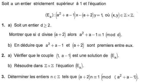
Soit un entier strictement supérieur à 1 et l'équation
1. a) Soit un entier Nous devons montrer que si divise , alors
Calcul préliminaire
Nous supposons que divise
Dans ce cas, divise , soit divise
Donc, , soit
Par conséquent, si divise , alors
1. b) Nous devons en déduire que et sont premiers entre eux.
Soit
Donc
Cela signifie que r divise 1.
Or r est un nombre entier strictement positif.
D'où
Par conséquent, et sont premiers entre eux.
2. a) Vérifions que le couple est une solution de
Par conséquent, le couple est une solution de
2. b) Résolvons dans l'équation
Soit une solution de l'équation
En utilisant la question 2. a), nous obtenons alors :
Donc divise
De plus, nous savons par la question 1. b) que et sont premiers entre eux.
Utilisons le lemme de Gauss (Si a, b et c sont des nombres entiers tels que a et b sont premiers entre eux et a divise bc, alors a divise c.)
Nous déduisons ainsi que divise
Dès lors ,
D'où,
Par conséquent, si est une solution de l'équation alors
Réciproquement, démontrons que pour tout entier k , les couples sont solutions de l'équation
En conclusion, l'ensemble des solutions dans de l'équation est
3. Nous devons déterminer les entiers tels que
Déterminons une valeur de n en calculant un inverse de modulo
Nous avons montré dans la question 2. a) que
D'où , soit
Dès lors, est un inverse de modulo
Nous obtenons ainsi :
En d'autres termes, les solutions de l'équation sont les nombres
Par conséquent, l'ensemble des entiers tels que est
6,5 points
exercice 4
Soit f la fonction définie sur [0 ; +[ par
On désigne par sa courbe représentative dans un repère
Partie A
1. a) Montrons que f est continue à droite en 0.
Par définition,
Calculons
Nous en déduisons que
Par conséquent, la fonction est continue à droite en 0.
1. b) Nous devons calculer
Interprétation graphique.
La fonction est définie en 0 et
Dès lors,
En conséquence, la fonction n'est pas dérivable à droite en 0.
De plus, la courbe possède une demi-tangente au point de coordonnées (0 ; 0) d'équation
Cette demi-tangente est orientée vers le haut.
2. Nous devons calculer et
Nous en déduisons que la courbe admet une branche parabolique de direction l'axe des abscisses au voisinage de +.
3. a) Montrons que pour tout
Pour tout
3. b) Dressons le tableau de variations de
4. Soit le point et la tangente à en
4. a) Déterminons une équation de la tangente
Une équation de la tangente est de la forme :
Or car le point de tangence est
Donc une équation de la tangente est de la forme : , soit
4. b) Ci-dessous le tableau de variation de la fonction sur ]0 ; +[.
Nous devons montrer que
Considérons la fonction définie sur [0 ; +[ par
Nous devons alors montrer que
La fonction est dérivable sur ]0 ; +[.
Pour tout x ]0 ; +[,
D'où le tableau de variation de la fonction sur ]0 ; +[ est le suivant :
Nous en déduisons que sur ]0 ; +[.
Dès lors, la fonction est strictement croissante sur [0 ; +[.
De plus,
Il s'ensuit que :
Si alors , soit Si alors , soit
D'où
Par conséquent, nous avons montré que
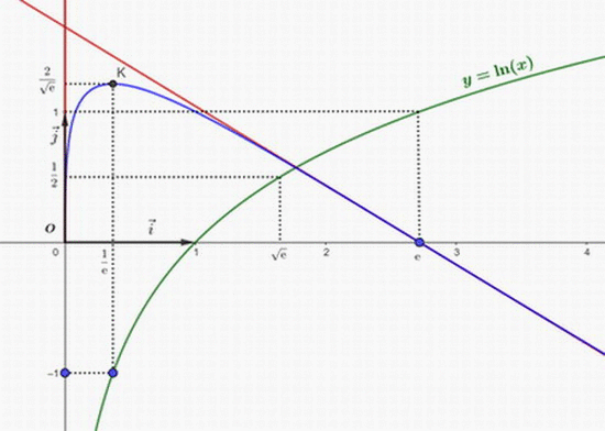
5. Dans la figure ci-dessous, nous avons représenté la courbe de la fonction logarithme népérien dans le repère
5. a) Plaçons le point dans le repère
Nous savons que .
Donc le point appartient à la courbe de la fonction logarithme népérien.
Autrement dit, est l'abscisse du point de la courbe de la fonction logarithme népérien dont l'ordonnée vaut -1.
Nous pouvons ainsi aisément fixer sur l'axe des abscisses.
De plus, l'ordonnée est fixée dans la figure de l'énoncé.
D'où la construction du point
Voir figure ci-dessous.
5. b) Traçons et dans ce repère.
Nous avons montré dans la question 3. b) que f admet un maximum égal à pour
Donc le point est un sommet de la courbe
Partie B
Soit
On considère les fonctions et définies sur respectivement par : et
1. Montrons que les fonctions et sont dérivables sur
Les fonctions et sont continues sur
Donc la fonction est continue sur
De plus,
Nous en déduisons que la fonction est dérivable sur
Les fonctions et sont continues sur
Donc la fonction est continue sur
De plus, la fonction est dérivable sur et
Nous en déduisons que la fonction est dérivable sur
2. Montrons que pour tout x > 0.
La fonction est dérivable sur et pour tout x > 0,
D'où pour tout x > 0.
De même, la fonction est dérivable sur et pour tout x > 0,
Dès lors, pour tout x > 0, où k est une constante réelle.
Si alors
Par conséquent, pour tout x > 0,
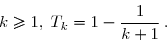
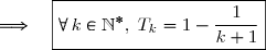
3. Soit la suite définie sur par
3. a) Nous devons montrer que pour tout
Soit
De plus,
Par conséquent,
3. b) Nous devons en déduire
Nous savons que
Selon le théorème d'encadrement (théorème des gendarmes), nous en déduisons que
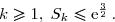
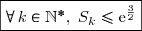
4. Soit les suites et définies par et
4. a) Nous devons montrer que pour tout entier
4. b) Nous devons montrer que pour tout entier
En utilisant les questions Partie B - 3. a) et 4. a), nous déduisons que pour tout
Par conséquent,
4. c) Nous devons en déduire que la suite est convergente vers un réel tel que
Montrons que la suite est croissante.
Or
D'où
Nous en déduisons que la suite est croissante.
De plus, la suite est majorée par
Par conséquent, la suite est convergente vers un réel
Montrons que
En utilisant la question Partie B - 3. a), nous obtenons :
Donc , soit
Publié par malou
le
ceci n'est qu'un extrait
Pour visualiser la totalité des cours vous devez vous inscrire / connecter (GRATUIT) Inscription Gratuitese connecter
Merci à Hiphigenie / malou pour avoir contribué à l'élaboration de cette fiche
Désolé, votre version d'Internet Explorer est plus que périmée ! Merci de le mettre à jour ou de télécharger Firefox ou Google Chrome pour utiliser le site. Votre ordinateur vous remerciera !
 est rapporté à un repère orthonormé direct
 \,.})
 et
et 
 on associe le point M' de
(z'-\text i)=1.})


(z'-\text i)=(z-\text i)\left(\dfrac{\text iz+2}{z-\text i}-\text i\right) \\ \overset{ { \white{ . } } } { \phantom{(z-\text i)(z'-\text i)}= (z-\text i)\dfrac{\text iz+2}{z-\text i}-(z-\text i)\text i } \\ \overset{ { \white{ . } } } { \phantom{(z-\text i)(z'-\text i)}=\text iz+2-\text iz+\text i^2 } \\ \overset{ { \white{ . } } } { \phantom{(z-\text i)(z'-\text i)}=2-1 } \\ \overset{ { \phantom{ . } } } { \phantom{(z-\text i)(z'-\text i)}=1 } \\\\\Longrightarrow\quad\boxed{\forall\,z\neq\text i,\;\;(z-\text i)(z'-\text i)=1})
(z'-\text i)=1\quad\Longrightarrow\quad (z-\text i)(z'-\text i)\neq0)

(z'-\text i)=1}\quad\Longrightarrow\quad z-\text i\neq0\quad\text{et}\quad z'-\text i\neq0 } \\ \overset{ { \white{ . } } } { \phantom{(z-\text i)(z'-\text i)=1}\quad\Longrightarrow\quad \boxed{z'\neq\text i }})
 tels que
=\text iz+2} \\ \overset{ { \white{ . } } } { \phantom{M=M'}\quad\Longleftrightarrow\quad z^2-\text iz=\text iz+2})

^2=1} \\ \overset{ { \phantom{ . } } } { \phantom{M=M'}\quad\Longleftrightarrow\quad z-\text i=1\quad\text{ou}\quad z-\text i=-1})

 est
est 
^2\in \R \,. })

^2}{(z'-\text i)(z-\text i)}\in\R} \\\overset{ { \white{ . } } } { { }\quad\Longleftrightarrow\quad \boxed{(z-\text i)^2\in\R}\quad\quad\text{car }(z'-\text i)(z-\text i)=1 \rightarrow\text {voir question }1.})

^2\in \R })
^2=k\pi\quad\quad\text{où }k\in\Z} \\\overset{ { \white{ . } } } { { \phantom{ WWWWwWiWWwwWWWWW } } \Longleftrightarrow\quad2\arg(z-\text i)=k\pi\quad\quad\text{où }k\in\Z})
=k\dfrac{\pi}{2}\quad\quad\text{où }k\in\Z} \\ { \white{ WWWWwWiWWwwWWWWW } } \overset{ { \phantom{ . } } } {\Longleftrightarrow\quad (\widehat{\overrightarrow{u},\overrightarrow{AM}})=k\dfrac{\pi}{2}\quad\quad\text{où }k\in\Z})
 ).
).  et
et ![(\widehat{\overrightarrow{AB},\overrightarrow{AM}})\equiv(\widehat{\overrightarrow{AM'},\overrightarrow{AB}})\,[2\pi].](https://latex.ilemaths.net/latex-0.tex? (\widehat{\overrightarrow{AB},\overrightarrow{AM}})\equiv(\widehat{\overrightarrow{AM'},\overrightarrow{AB}})\,[2\pi]. )
(z'-\text i)| } \\ \overset{ { \white{ . } } } { \phantom{AM\times AM',u}=|1|\quad(\text{voir question 1.)} })
![{\bullet}{\white{x}}(\widehat{\overrightarrow{AB},\overrightarrow{AM}})\equiv\arg\left(\dfrac{z-\text i}{(1+\text i)-\text i}\right)\,[2\pi] \\\overset{ { \white{ . } } } { \phantom{WWWWWi}\equiv\arg\left(\dfrac{z-\text i}{1}\right)\,[2\pi]} \\\overset{ { \white{ . } } } { \phantom{WWWWWi}\equiv\arg\left(z-\text i\right)\,[2\pi]}](https://latex.ilemaths.net/latex-0.tex?{\bullet}{\white{x}}(\widehat{\overrightarrow{AB},\overrightarrow{AM}})\equiv\arg\left(\dfrac{z-\text i}{(1+\text i)-\text i}\right)\,[2\pi] \\\overset{ { \white{ . } } } { \phantom{WWWWWi}\equiv\arg\left(\dfrac{z-\text i}{1}\right)\,[2\pi]} \\\overset{ { \white{ . } } } { \phantom{WWWWWi}\equiv\arg\left(z-\text i\right)\,[2\pi]} )
![\\\overset{ { \white{ . } } } { \phantom{WWWWWi}\equiv\arg\left(\dfrac{1}{z'-\text i}\right)\, [2\pi]\quad(\text{voir question 1.)} } \\\overset{ { \white{ . } } } { \phantom{WWWWWi}\equiv\arg\left(\dfrac{(1+\text i)-\text i}{z'-\text i}\right)\, [2\pi]} \\\overset{ { \phantom{ . } } } { \phantom{WWWWWi}\equiv(\widehat{\overrightarrow{AM'},\overrightarrow{AB}})\,[2\pi].} \\\\\Longrightarrow\quad\boxed{(\widehat{\overrightarrow{AB},\overrightarrow{AM}})\equiv(\widehat{\overrightarrow{AM'},\overrightarrow{AB}})\,[2\pi] }](https://latex.ilemaths.net/latex-0.tex?\\\overset{ { \white{ . } } } { \phantom{WWWWWi}\equiv\arg\left(\dfrac{1}{z'-\text i}\right)\, [2\pi]\quad(\text{voir question 1.)} } \\\overset{ { \white{ . } } } { \phantom{WWWWWi}\equiv\arg\left(\dfrac{(1+\text i)-\text i}{z'-\text i}\right)\, [2\pi]} \\\overset{ { \phantom{ . } } } { \phantom{WWWWWi}\equiv(\widehat{\overrightarrow{AM'},\overrightarrow{AB}})\,[2\pi].} \\\\\Longrightarrow\quad\boxed{(\widehat{\overrightarrow{AB},\overrightarrow{AM}})\equiv(\widehat{\overrightarrow{AM'},\overrightarrow{AB}})\,[2\pi] })

 est le cercle de centre A et de rayon 1.
 et
et 
 .
. }) .
. nous savons par la question 5 que
  et
et ![(\widehat{\overrightarrow{AB},\overrightarrow{AK}})\equiv(\widehat{\overrightarrow{AK'},\overrightarrow{AB}})\,[2\pi].](https://latex.ilemaths.net/latex-0.tex? (\widehat{\overrightarrow{AB},\overrightarrow{AK}})\equiv(\widehat{\overrightarrow{AK'},\overrightarrow{AB}})\,[2\pi]. )
-\text i } \\\overset{ { \white{ . } } } { \phantom{WWW} = \text e^{\text i\frac{\pi}{4}} } )
![\left\lbrace\begin{matrix}AK=|z_K-z_A|=\left|\text e^{\text i\frac{\pi}{4}}\right|\\\\ \left(\widehat{\overrightarrow{u}\,,\,\overrightarrow{AK}}\right)\equiv\arg\left(\text e^{\text i\frac{\pi}{4}}\right)\,[2\pi]\end{matrix}\right.\quad\Longrightarrow\quad\left\lbrace\begin{matrix}AK=1\\\\\left(\widehat{\overrightarrow{u}\,,\,\overrightarrow{AK}}\right)\equiv\dfrac{\pi}{4}\,[2\pi]\end{matrix}\right.](https://latex.ilemaths.net/latex-0.tex?\left\lbrace\begin{matrix}AK=|z_K-z_A|=\left|\text e^{\text i\frac{\pi}{4}}\right|\\\\ \left(\widehat{\overrightarrow{u}\,,\,\overrightarrow{AK}}\right)\equiv\arg\left(\text e^{\text i\frac{\pi}{4}}\right)\,[2\pi]\end{matrix}\right.\quad\Longrightarrow\quad\left\lbrace\begin{matrix}AK=1\\\\\left(\widehat{\overrightarrow{u}\,,\,\overrightarrow{AK}}\right)\equiv\dfrac{\pi}{4}\,[2\pi]\end{matrix}\right.)

![\text{et }\;(\widehat{\overrightarrow{AB},\overrightarrow{AK}})\equiv(\widehat{\overrightarrow{AK'},\overrightarrow{AB}})\,[2\pi]\quad\Longleftrightarrow\quad(\widehat{\overrightarrow{u},\overrightarrow{AK}})\equiv(\widehat{\overrightarrow{AK'},\overrightarrow{AB}})\,[2\pi] \\\overset{ { \white{ . } } } {\phantom{WWWWWWWWWWwWW} \quad\Longleftrightarrow\quad(\widehat{\overrightarrow{AB},\overrightarrow{AK'}})\equiv-(\widehat{\overrightarrow{u},\overrightarrow{AK}})\,[2\pi] } \\\overset{ { \white{ . } } } {\phantom{WWWWWWWWWWwWW} \quad\Longleftrightarrow\quad\boxed{(\widehat{\overrightarrow{AB},\overrightarrow{AK'}})\equiv-\dfrac{\pi}{4}\,[2\pi]}}](https://latex.ilemaths.net/latex-0.tex?\text{et }\;(\widehat{\overrightarrow{AB},\overrightarrow{AK}})\equiv(\widehat{\overrightarrow{AK'},\overrightarrow{AB}})\,[2\pi]\quad\Longleftrightarrow\quad(\widehat{\overrightarrow{u},\overrightarrow{AK}})\equiv(\widehat{\overrightarrow{AK'},\overrightarrow{AB}})\,[2\pi] \\\overset{ { \white{ . } } } {\phantom{WWWWWWWWWWwWW} \quad\Longleftrightarrow\quad(\widehat{\overrightarrow{AB},\overrightarrow{AK'}})\equiv-(\widehat{\overrightarrow{u},\overrightarrow{AK}})\,[2\pi] } \\\overset{ { \white{ . } } } {\phantom{WWWWWWWWWWwWW} \quad\Longleftrightarrow\quad\boxed{(\widehat{\overrightarrow{AB},\overrightarrow{AK'}})\equiv-\dfrac{\pi}{4}\,[2\pi]}})

![\overset{ { \white{ . } } } { \left(\widehat{\overrightarrow{AB}\,,\,\overrightarrow{AM}}\right)\equiv\dfrac{\pi}{4}\,[2\pi]. }](https://latex.ilemaths.net/latex-0.tex?\overset{ { \white{ . } } } { \left(\widehat{\overrightarrow{AB}\,,\,\overrightarrow{AM}}\right)\equiv\dfrac{\pi}{4}\,[2\pi]. })
![\left\lbrace\begin{matrix}(\widehat{\overrightarrow{AB},\overrightarrow{AM}})\equiv(\widehat{\overrightarrow{AM'},\overrightarrow{AB}})\,[2\pi]\\\\\overset{ { \white{ . } } } { \left(\widehat{\overrightarrow{AB}\,,\,\overrightarrow{AM}}\right)\equiv\dfrac{\pi}{4}\,[2\pi]. } \end{matrix}\right.\quad\Longrightarrow\quad(\widehat{\overrightarrow{AM'},\overrightarrow{AB}})\equiv\dfrac{\pi}{4}\,[2\pi] \\\overset{ { \white{ . } } } {\phantom{WWWWWWWWWWwWW} \quad\Longrightarrow\quad(\widehat{\overrightarrow{AB},\overrightarrow{AM'}})\equiv-\dfrac{\pi}{4}\,[2\pi] }](https://latex.ilemaths.net/latex-0.tex?\left\lbrace\begin{matrix}(\widehat{\overrightarrow{AB},\overrightarrow{AM}})\equiv(\widehat{\overrightarrow{AM'},\overrightarrow{AB}})\,[2\pi]\\\\\overset{ { \white{ . } } } { \left(\widehat{\overrightarrow{AB}\,,\,\overrightarrow{AM}}\right)\equiv\dfrac{\pi}{4}\,[2\pi]. } \end{matrix}\right.\quad\Longrightarrow\quad(\widehat{\overrightarrow{AM'},\overrightarrow{AB}})\equiv\dfrac{\pi}{4}\,[2\pi] \\\overset{ { \white{ . } } } {\phantom{WWWWWWWWWWwWW} \quad\Longrightarrow\quad(\widehat{\overrightarrow{AB},\overrightarrow{AM'}})\equiv-\dfrac{\pi}{4}\,[2\pi] })


 et par la question 7. a) que
![\left\lbrace\begin{matrix}\left(\widehat{\overrightarrow{AB},\overrightarrow{AE}}\right)\equiv\left(\widehat{\overrightarrow{AB},\overrightarrow{AQ}}\right)\equiv\dfrac{\pi}{4}\,[2\pi]\\\overset{ { \white{ . } } } { \left(\widehat{\overrightarrow{AB},\overrightarrow{AQ'}}\right)\equiv-\dfrac{\pi}{4}\,[2\pi]}\phantom{WWWWW}\end{matrix}\right.\quad\Longrightarrow\quad\boxed{\left\lbrace\begin{matrix}\left(\widehat{\overrightarrow{AB},\overrightarrow{AE}}\right)\equiv\dfrac{\pi}{4}\,[2\pi]\\\overset{ { \white{ . } } } { \left(\widehat{\overrightarrow{AB},\overrightarrow{AQ'}}\right)\equiv-\dfrac{\pi}{4}\,[2\pi]}\end{matrix}\right.}](https://latex.ilemaths.net/latex-0.tex?\left\lbrace\begin{matrix}\left(\widehat{\overrightarrow{AB},\overrightarrow{AE}}\right)\equiv\left(\widehat{\overrightarrow{AB},\overrightarrow{AQ}}\right)\equiv\dfrac{\pi}{4}\,[2\pi]\\\overset{ { \white{ . } } } { \left(\widehat{\overrightarrow{AB},\overrightarrow{AQ'}}\right)\equiv-\dfrac{\pi}{4}\,[2\pi]}\phantom{WWWWW}\end{matrix}\right.\quad\Longrightarrow\quad\boxed{\left\lbrace\begin{matrix}\left(\widehat{\overrightarrow{AB},\overrightarrow{AE}}\right)\equiv\dfrac{\pi}{4}\,[2\pi]\\\overset{ { \white{ . } } } { \left(\widehat{\overrightarrow{AB},\overrightarrow{AQ'}}\right)\equiv-\dfrac{\pi}{4}\,[2\pi]}\end{matrix}\right.})
 ABC est un triangle rectangle isocèle en A .
 et
et ![\overset{ { \white{ . } } } { \left(\widehat{\overrightarrow{CA},\overrightarrow{CD}}\right)\equiv\dfrac{5\pi}{6}\,[2\pi]. }](https://latex.ilemaths.net/latex-0.tex?\overset{ { \white{ . } } } { \left(\widehat{\overrightarrow{CA},\overrightarrow{CD}}\right)\equiv\dfrac{5\pi}{6}\,[2\pi]. })
 et que
 car ABC est un triangle.


. })
![\left(\widehat{\overrightarrow{AB},\overrightarrow{BE}}\right)\equiv\left(\widehat{\overrightarrow{AB},\overrightarrow{CD}}\right)\,[2\pi] \\\overset{ { \white{ . } } } { \phantom{\left(\widehat{\overrightarrow{AB},\overrightarrow{BE}}\right)} \equiv\left(\widehat{\overrightarrow{AB},\overrightarrow{AC}}\right)+\left(\widehat{\overrightarrow{AC},\overrightarrow{CD}}\right)\,[2\pi] } \\\overset{ { \white{ . } } } { \phantom{\left(\widehat{\overrightarrow{AB},\overrightarrow{BE}}\right)} \equiv\left(\widehat{\overrightarrow{AB},\overrightarrow{AC}}\right)+\left(\widehat{\overrightarrow{CA},\overrightarrow{CD}}\right)+\pi\,[2\pi] } \\\overset{ { \white{ . } } } { \phantom{\left(\widehat{\overrightarrow{AB},\overrightarrow{BE}}\right)} \equiv\dfrac{\pi}{2}+\dfrac{5\pi}{6}+\pi\,[2\pi] }](https://latex.ilemaths.net/latex-0.tex?\left(\widehat{\overrightarrow{AB},\overrightarrow{BE}}\right)\equiv\left(\widehat{\overrightarrow{AB},\overrightarrow{CD}}\right)\,[2\pi] \\\overset{ { \white{ . } } } { \phantom{\left(\widehat{\overrightarrow{AB},\overrightarrow{BE}}\right)} \equiv\left(\widehat{\overrightarrow{AB},\overrightarrow{AC}}\right)+\left(\widehat{\overrightarrow{AC},\overrightarrow{CD}}\right)\,[2\pi] } \\\overset{ { \white{ . } } } { \phantom{\left(\widehat{\overrightarrow{AB},\overrightarrow{BE}}\right)} \equiv\left(\widehat{\overrightarrow{AB},\overrightarrow{AC}}\right)+\left(\widehat{\overrightarrow{CA},\overrightarrow{CD}}\right)+\pi\,[2\pi] } \\\overset{ { \white{ . } } } { \phantom{\left(\widehat{\overrightarrow{AB},\overrightarrow{BE}}\right)} \equiv\dfrac{\pi}{2}+\dfrac{5\pi}{6}+\pi\,[2\pi] } )
![\\\overset{ { \phantom{ . } } } { \phantom{\left(\widehat{\overrightarrow{AB},\overrightarrow{BE}}\right)} \equiv\dfrac{7\pi}{3}\,[2\pi] } \\\overset{ { \phantom{ . } } } { \phantom{\left(\widehat{\overrightarrow{AB},\overrightarrow{BE}}\right)} \equiv\dfrac{\pi}{3}\,[2\pi] } \\\\\Longrightarrow\quad\boxed{\left(\widehat{\overrightarrow{AB},\overrightarrow{BE}}\right)\equiv\dfrac{\pi}{3}\,[2\pi] }](https://latex.ilemaths.net/latex-0.tex?\\\overset{ { \phantom{ . } } } { \phantom{\left(\widehat{\overrightarrow{AB},\overrightarrow{BE}}\right)} \equiv\dfrac{7\pi}{3}\,[2\pi] } \\\overset{ { \phantom{ . } } } { \phantom{\left(\widehat{\overrightarrow{AB},\overrightarrow{BE}}\right)} \equiv\dfrac{\pi}{3}\,[2\pi] } \\\\\Longrightarrow\quad\boxed{\left(\widehat{\overrightarrow{AB},\overrightarrow{BE}}\right)\equiv\dfrac{\pi}{3}\,[2\pi] } )

=B }) et que
et que =E. })
![f(A)=B\quad\Longleftrightarrow\quad\left\lbrace\begin{matrix}OA=OB\\\overset{ { \white{ . } } } { \left(\widehat{\overrightarrow{OA}\,,\,\overrightarrow{OB}}\right)\equiv\dfrac{\pi}{3}\,[2\pi]}\end{matrix}\right.](https://latex.ilemaths.net/latex-0.tex?f(A)=B\quad\Longleftrightarrow\quad\left\lbrace\begin{matrix}OA=OB\\\overset{ { \white{ . } } } { \left(\widehat{\overrightarrow{OA}\,,\,\overrightarrow{OB}}\right)\equiv\dfrac{\pi}{3}\,[2\pi]}\end{matrix}\right.)
![f(B)=E\quad\Longleftrightarrow\quad\left\lbrace\begin{matrix}OB=OE\\\overset{ { \white{ . } } } { \left(\widehat{\overrightarrow{OB}\,,\,\overrightarrow{OE}}\right)\equiv\dfrac{\pi}{3}\,[2\pi]}\end{matrix}\right.](https://latex.ilemaths.net/latex-0.tex?f(B)=E\quad\Longleftrightarrow\quad\left\lbrace\begin{matrix}OB=OE\\\overset{ { \white{ . } } } { \left(\widehat{\overrightarrow{OB}\,,\,\overrightarrow{OE}}\right)\equiv\dfrac{\pi}{3}\,[2\pi]}\end{matrix}\right.)

 et d'angle

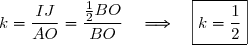
=I\\\overset{ { \white{ . } } } {S(O)=J}\end{matrix}\right.\quad\Longrightarrow\quad k=\dfrac{IJ}{AO})


![\theta\equiv\left(\widehat{\overrightarrow{AO}\,,\,\overrightarrow{IJ}}\right)\,[2\pi] \\\overset{ { \white{ . } } } {\phantom{\theta}\equiv\left(\widehat{\overrightarrow{AO}\,,\,\overrightarrow{BO}}\right)\,[2\pi] } \\\overset{ { \white{ . } } } {\phantom{\theta}\equiv\left(\widehat{\overrightarrow{OA}\,,\,\overrightarrow{OB}}\right)\,[2\pi] } \\\overset{ { \white{ . } } } {\phantom{\theta}\equiv\dfrac{\pi}{3}\,[2\pi] } \\\\\Longrightarrow\boxed{\theta\equiv\dfrac{\pi}{3}\,[2\pi] }](https://latex.ilemaths.net/latex-0.tex?\theta\equiv\left(\widehat{\overrightarrow{AO}\,,\,\overrightarrow{IJ}}\right)\,[2\pi] \\\overset{ { \white{ . } } } {\phantom{\theta}\equiv\left(\widehat{\overrightarrow{AO}\,,\,\overrightarrow{BO}}\right)\,[2\pi] } \\\overset{ { \white{ . } } } {\phantom{\theta}\equiv\left(\widehat{\overrightarrow{OA}\,,\,\overrightarrow{OB}}\right)\,[2\pi] } \\\overset{ { \white{ . } } } {\phantom{\theta}\equiv\dfrac{\pi}{3}\,[2\pi] } \\\\\Longrightarrow\boxed{\theta\equiv\dfrac{\pi}{3}\,[2\pi] })
 et d'angle

 }) et
et . })
=(S\circ f^{-1})(O) \\\overset{ { \white{ . } } } { \phantom{\bullet{\phantom{x}} h(O)}=S(f^{-1}(O)) } \\\overset{ { \white{ . } } } { \phantom{ \bullet{\phantom{x}}h(O)}=S(O) } \\\overset{ { \white{ . } } } { \phantom{\bullet{\phantom{x}} h(O)}=J } \\\\\Longrightarrow\boxed{h(O)=J} )
=(S\circ f^{-1})(B) \\\overset{ { \white{ . } } } { \phantom{\bullet{\phantom{x}} h(O)}=S(f^{-1}(B)) } \\\overset{ { \white{ . } } } { \phantom{ \bullet{\phantom{x}}h(O)}=S(A) } \\\overset{ { \white{ . } } } { \phantom{\bullet{\phantom{x}} h(O)}=I } \\\\\Longrightarrow\boxed{h(B)=I} )

 et
et  sont des similitudes directes de rapports respectifs
  et 1 et d'angles respectifs
  et
et 
 est une similitude directe de rapport
  et d'angle
=J }) et
et  =I})
 le milieu du segment [LD ].
 car CBED est un parallélogramme.
 car OABE est un losange.
![\overset{ { \white{ . } } } { \left(\widehat{\overrightarrow{DC},\overrightarrow{DO}}\right)\equiv\dfrac{\pi}{6}\,[2\pi]. }](https://latex.ilemaths.net/latex-0.tex?\overset{ { \white{ . } } } { \left(\widehat{\overrightarrow{DC},\overrightarrow{DO}}\right)\equiv\dfrac{\pi}{6}\,[2\pi]. })
![\left(\widehat{\overrightarrow{DC},\overrightarrow{DO}}\right)\equiv\left(\widehat{\overrightarrow{DC},\overrightarrow{CA}}\right)\,[2\pi] \\\overset{ { \white{ . } } } {\phantom{WWWWW}\equiv-\left(\widehat{\overrightarrow{CA},\overrightarrow{DC}}\right)\,[2\pi] } \\\overset{ { \white{ . } } } {\phantom{WWWWW}\equiv-\left(\widehat{\overrightarrow{CA},\overrightarrow{CD}}\right)+\pi\,[2\pi] } \\\overset{ { \white{ . } } } {\phantom{WWWWW}\equiv-\dfrac{5\pi}{6}+\pi\,[2\pi] } \\\overset{ { \phantom{ . } } } {\phantom{WWWWW}\equiv\dfrac{\pi}{6}\,[2\pi] } \\\\\Longrightarrow\quad\boxed{\left(\widehat{\overrightarrow{DC},\overrightarrow{DO}}\right)\equiv\dfrac{\pi}{6}\,[2\pi]}](https://latex.ilemaths.net/latex-0.tex?\left(\widehat{\overrightarrow{DC},\overrightarrow{DO}}\right)\equiv\left(\widehat{\overrightarrow{DC},\overrightarrow{CA}}\right)\,[2\pi] \\\overset{ { \white{ . } } } {\phantom{WWWWW}\equiv-\left(\widehat{\overrightarrow{CA},\overrightarrow{DC}}\right)\,[2\pi] } \\\overset{ { \white{ . } } } {\phantom{WWWWW}\equiv-\left(\widehat{\overrightarrow{CA},\overrightarrow{CD}}\right)+\pi\,[2\pi] } \\\overset{ { \white{ . } } } {\phantom{WWWWW}\equiv-\dfrac{5\pi}{6}+\pi\,[2\pi] } \\\overset{ { \phantom{ . } } } {\phantom{WWWWW}\equiv\dfrac{\pi}{6}\,[2\pi] } \\\\\Longrightarrow\quad\boxed{\left(\widehat{\overrightarrow{DC},\overrightarrow{DO}}\right)\equiv\dfrac{\pi}{6}\,[2\pi]})
=L. })
 et que
 ![\overset{ { \white{ . } } } { \left(\widehat{\overrightarrow{O\Omega},\overrightarrow{OL}}\right)\equiv\dfrac{\pi}{3}\,[2\pi]\,. }](https://latex.ilemaths.net/latex-0.tex?\overset{ { \white{ . } } } { \left(\widehat{\overrightarrow{O\Omega},\overrightarrow{OL}}\right)\equiv\dfrac{\pi}{3}\,[2\pi]\,. })
 est équilatéral.
![\left(\widehat{\overrightarrow{\Omega L},\overrightarrow{\Omega O}}\right)\equiv2\left(\widehat{\overrightarrow{D L},\overrightarrow{D O}}\right)\,[2\pi].](https://latex.ilemaths.net/latex-0.tex?\left(\widehat{\overrightarrow{\Omega L},\overrightarrow{\Omega O}}\right)\equiv2\left(\widehat{\overrightarrow{D L},\overrightarrow{D O}}\right)\,[2\pi].)
![\text{D'où }\;\left(\widehat{\overrightarrow{\Omega L},\overrightarrow{\Omega O}}\right)\equiv2\left(\widehat{\overrightarrow{D L},\overrightarrow{D O}}\right)\,[2\pi] \\\overset{ { \white{ . } } } {\phantom{WWWWWWW} \equiv2\left(\widehat{\overrightarrow{D C},\overrightarrow{D O}}\right)\,[2\pi] } \\\overset{ { \white{ . } } } {\phantom{WWWWWWW} \equiv2\times\dfrac{\pi}{6}\,[2\pi] \quad\quad(\text{voir 4. b)} } \\\overset{ { \white{ . } } } {\phantom{WWWWWWW} \equiv\dfrac{\pi}{3}\,[2\pi] } \\\\\Longrightarrow\quad \boxed{\left(\widehat{\overrightarrow{\Omega L},\overrightarrow{\Omega O}}\right)\equiv\dfrac{\pi}{3}\,[2\pi] }](https://latex.ilemaths.net/latex-0.tex?\text{D'où }\;\left(\widehat{\overrightarrow{\Omega L},\overrightarrow{\Omega O}}\right)\equiv2\left(\widehat{\overrightarrow{D L},\overrightarrow{D O}}\right)\,[2\pi] \\\overset{ { \white{ . } } } {\phantom{WWWWWWW} \equiv2\left(\widehat{\overrightarrow{D C},\overrightarrow{D O}}\right)\,[2\pi] } \\\overset{ { \white{ . } } } {\phantom{WWWWWWW} \equiv2\times\dfrac{\pi}{6}\,[2\pi] \quad\quad(\text{voir 4. b)} } \\\overset{ { \white{ . } } } {\phantom{WWWWWWW} \equiv\dfrac{\pi}{3}\,[2\pi] } \\\\\Longrightarrow\quad \boxed{\left(\widehat{\overrightarrow{\Omega L},\overrightarrow{\Omega O}}\right)\equiv\dfrac{\pi}{3}\,[2\pi] })
 et
et ![\left(\widehat{\overrightarrow{\Omega L},\overrightarrow{\Omega O}}\right)\equiv\dfrac{\pi}{3}\,[2\pi]](https://latex.ilemaths.net/latex-0.tex?\left(\widehat{\overrightarrow{\Omega L},\overrightarrow{\Omega O}}\right)\equiv\dfrac{\pi}{3}\,[2\pi]) , il s'ensuit que le triangle
, il s'ensuit que le triangle  et
et ![\left(\widehat{\overrightarrow{O\Omega },\overrightarrow{OL}}\right)\equiv\dfrac{\pi}{3}\,[2\pi]](https://latex.ilemaths.net/latex-0.tex?\left(\widehat{\overrightarrow{O\Omega },\overrightarrow{OL}}\right)\equiv\dfrac{\pi}{3}\,[2\pi])
=L}\,. })
=\Omega\,. })
 soit
soit 
=(h\circ f)(\Omega) \\\overset{ { \white{ . } } } { \phantom{S(\Omega)}=h(f(\Omega) ) } \\\overset{ { \white{ . } } } { \phantom{S(\Omega)}=h(L) } \\\overset{ { \white{ . } } } { \phantom{S(\Omega)}=\Omega } \\\\\Longrightarrow\quad\boxed{S(\Omega)=\Omega})
. })
 \\\overset{ { \white{ . } } } { \phantom{K}=(h\circ f)(B) } \\\overset{ { \white{ . } } } { \phantom{K}=h(f(B) ) } \\\\\Longrightarrow \quad K=h(f(B) ) )
=E })
 ) \\\overset{ { \white{ . } } } { f(B)=E\phantom{xxx}} \end{matrix}\right.\quad\Longrightarrow\boxed{K=h(E)})
 nous en déduisons que
=L }) (voir question 4. c)
(voir question 4. c)}}. })
 nous obtenons :
 )=(OE). })
=f^{-1}((OE))}}. })
\quad\Longrightarrow\quad f^{-1}(L)\in f^{-1}((OE)) \\\overset{ { \white{ . } } } { \phantom{\text{D'où }\; L\in(OE)}\quad\Longrightarrow\quad \boxed{\Omega\in (OB)} } )
. })
. })
=\Omega\\\overset{ { \white{ . } } } { S(O)=J }\\\overset{ { \white{ . } } } { S(B)=K } \end{matrix}\right.)
\quad\Longrightarrow\quad S(\Omega)\in S((OB)) \\\overset{ { \white{ . } } } { \phantom{\text{D'où }\; L\in(OE)}\quad\Longrightarrow\quad \boxed{\Omega\in (JK)} } )
![\overset{ { \white{ . } } } { \left(\widehat{\overrightarrow{OB},\overrightarrow{JK}}\right) \equiv\dfrac{\pi}{3}\,[2\pi].}](https://latex.ilemaths.net/latex-0.tex?\overset{ { \white{ . } } } { \left(\widehat{\overrightarrow{OB},\overrightarrow{JK}}\right) \equiv\dfrac{\pi}{3}\,[2\pi].})
 et montrons que
![\overset{ { \white{ . } } } { \left(\widehat{\overrightarrow{\Omega A},\overrightarrow{\Omega I}}\right)=\dfrac{\pi}{3}\,[2\pi]}](https://latex.ilemaths.net/latex-0.tex?\overset{ { \white{ . } } } { \left(\widehat{\overrightarrow{\Omega A},\overrightarrow{\Omega I}}\right)=\dfrac{\pi}{3}\,[2\pi]}) car
car )=(\Omega I).})

=\Omega I\quad\Longrightarrow\quad \Omega I=\dfrac 1 2 \,\Omega A \\\overset{ { \white{ . } } } { \phantom{\text{D'où }\;S(\Omega A)=\Omega I}\quad\Longrightarrow\quad \Omega A=2 \,\Omega I } )

 sont alignés.
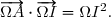
\cdot\overrightarrow{\Omega I}=0 } \\\overset{ { \white{ . } } } { \phantom{WWWWWW}\quad\Longleftrightarrow\quad \boxed{\overrightarrow{IA}\cdot\overrightarrow{\Omega I}=0 } })
 car
car 
 appartient à (IG ).
 un entier strictement supérieur à 1 et l'équation
:(a^2+a-1)x-(a+2)y=1,\;\text{ où }\;(x,y)\in\Z\times\Z. })

 Nous devons montrer que si
  divise
  }) , alors
, alors . })
(a-1)=a^2-a+2a-2 \\\overset{ { \white{ . } } } { \phantom{(a+2)(a-1)}=a^2+a-2 } \\\\\Longrightarrow\boxed{(a+2)(a-1)=a^2+a-2})
. })
(a-1) }) , soit
, soit 
}) , soit
, soit })
 et
et ) sont premiers entre eux.
sont premiers entre eux., \quad (r\in\N^*).)
 \\\overset{ { \white{ . } } } {\phantom{ r|a+2}\quad\Longrightarrow\quad a^2+a-1\equiv 1\;(\text{mod }r)\quad\text{(voir exercice 1. a)}} \\\\ {\bullet}{\white{x}}r|a^2+a-1\quad\Longrightarrow\quad a^2+a-1\equiv 0\;(\text{mod }r))
\\a^2+a-1\equiv 0\;(\text{mod }r)\end{matrix}\right.\quad\Longrightarrow\quad1\equiv0\;(\text{mod }r)})

}) sont premiers entre eux.
sont premiers entre eux. }) est une solution de
est une solution de . })
\times1-(a+2)(a-1)=a^2+a-1-(a^2+a-2) \\\phantom{(a^2+a-1)\times1-(a+2)(a-1)}=a^2+a-1-a^2-a+2 \\\phantom{(a^2+a-1)\times1-(a+2)(a-1)}=1)
 l'équation
 \in\Z\times\Z }) une solution de l'équation
une solution de l'équation x-(a+2)y=1\quad\Longleftrightarrow\quad (a^2+a-1)x-(a+2)y=(a^2+a-1)\times1-(a+2)(a-1) \\\overset{ { \white{ . } } } { \phantom{(a^2+a-1)x-(a+2)y=1}\quad\Longleftrightarrow\quad (a^2+a-1)x-(a^2+a-1)\times1=(a+2)y-(a+2)(a-1) } \\\overset{ { \white{ . } } } { \phantom{(a^2+a-1)x-(a+2)y=1}\quad\Longleftrightarrow\quad (a^2+a-1)(x-1)=(a+2)(y-a+1) })
(x-1). })
. })
k. }) D'où,
D'où, (x-1)=(a+2)(y-a+1) \\x-1=(a+2)k\quad(k\in\Z)\phantom{WWWWW} \end{matrix}\right.\quad\Longrightarrow\quad (a^2+a-1)(a+2)k=(a+2)(y-a+1)\;\;(k\in\Z) \\\phantom{WWWWWWWWWWWWWWWWW}\quad\Longrightarrow\quad (a^2+a-1)k=y-a+1\;\;(k\in\Z) \\\phantom{WWWWWWWWWWWWWWWWW}\quad\Longrightarrow\quad y=a-1+(a^2+a-1)k\;\;(k\in\Z))
, }) alors
alors k\phantom{XXXX}\\y=a-1+(a^2+a-1)k\end{matrix}\right.})
=\left(\overset{}{1+(a+2)k,a-1+(a^2+a-1)k}\right) }) sont solutions de l'équation
sont solutions de l'équation 
![(a^2+a-1)[1+(a+2)k]-(a+2)[a-1+(a^2+a-1)k] \\\overset{ { \white{ . } } } { \phantom{xxx}=(a^2+a-1)\times1{\blue{\,+\,(a^2+a-1)(a+2)k}}-(a+2)(a-1){\blue{\,-\,(a+2)(a^2+a-1)k }}} \\\overset{ { \white{ . } } } { \phantom{xxx}=(a^2+a-1)-(a+2)(a-1) } \\\overset{ { \white{ . } } } { \phantom{xxx}=1}](https://latex.ilemaths.net/latex-0.tex?(a^2+a-1)[1+(a+2)k]-(a+2)[a-1+(a^2+a-1)k] \\\overset{ { \white{ . } } } { \phantom{xxx}=(a^2+a-1)\times1{\blue{\,+\,(a^2+a-1)(a+2)k}}-(a+2)(a-1){\blue{\,-\,(a+2)(a^2+a-1)k }}} \\\overset{ { \white{ . } } } { \phantom{xxx}=(a^2+a-1)-(a+2)(a-1) } \\\overset{ { \white{ . } } } { \phantom{xxx}=1})
 }) est
est k,a-1+(a^2+a-1)k)\;/\;k\in\Z\rbrace} })
 tels que
 n\equiv1\;(\text{mod}\;(a^2+a-1)) })
 modulo
\times1-(a+2)(a-1)=1. })
(1-a)=1+(a^2+a-1)\times(-1)) , soit
, soit (1-a)\equiv1\;(\text{mod}\;(a^2+a-1)))
 est un inverse de
n\equiv1\;(\text{mod}\;(a^2+a-1))\quad\Longleftrightarrow\quad(1-a)(a+2)n\equiv1-a\;(\text{mod}\;(a^2+a-1)) \\\overset{ { \white{ . } } } { \phantom{(a+2)n\equiv1\;(\text{mod}\;(a^2+a-1))} \quad\Longleftrightarrow\quad n\equiv1-a\;(\text{mod}\;(a^2+a-1)) })
+(a^2+a-1)k\quad \text{avec }k\in\Z. })
+(a^2+a-1)k\;,\; k\in\Z\rbrace}\,. })
 [ par
[ par =\sqrt x(1-\ln x)\quad\text{si }x>0\\\overset{ { \white{ . } } } { f(0)=0 } \phantom{WWWWWWWWW}\end{matrix}\right. })
 sa courbe représentative dans un repère
 . })
 Par définition,
 =0 })
.})
=\lim\limits_{x\to 0^+}\sqrt x\,(1-\ln x) \\ \overset{ { \white{ . } } } { \phantom{WWWWi}=\lim\limits_{x\to 0^+}}(\sqrt x-\sqrt x\ln x) \\ \overset{ { \white{ . } } } { \phantom{WWWWi}=\lim\limits_{x\to 0^+}}\sqrt x-\lim\limits_{x\to 0^+}\sqrt x\ln x \\ \overset{ { \white{ . } } } { \phantom{WWWWi}=0-\lim\limits_{x\to 0^+}\sqrt x\ln x} \\ \overset{ { \phantom{ . } } } { \phantom{WWWWi}=-\lim\limits_{x\to 0^+}\sqrt x\ln x})
 }} \\ \overset{ { \white{ . } } } { \phantom{WWWWi}=0} \\\\\Longrightarrow\quad \lim\limits_{x\to 0^+}f(x)=0 )
=f(0)}\,.})
 est continue à droite en 0.
}{x}. )
}{x}=\lim\limits_{x\to0^+}\dfrac{\sqrt x(1-\ln x)}{x} \\\overset{ { \white{ . } } } { \phantom{ \lim\limits_{x\to0^+}\dfrac{f(x)}{x}}=\lim\limits_{x\to0^+}\dfrac{1-\ln x}{\sqrt x} } \\\\\text{Or }\;\left\lbrace\begin{matrix}\lim\limits_{x\to0^+}\ln x=-\infty\\\overset{ { \white{ . } } } { \lim\limits_{x\to0^+}\sqrt x=0^+\quad} \end{matrix}\right.\quad\Longrightarrow\quad\left\lbrace\begin{matrix}\lim\limits_{x\to0^+}1-\ln x=+\infty\\\overset{ { \white{ . } } } { \lim\limits_{x\to0^+}\sqrt x=0^+\quad} \end{matrix}\right. \\\\\phantom{\text{Or }\;WWwWWWWW}\quad\Longrightarrow\quad\lim\limits_{x\to0^+}\dfrac{1-\ln x}{\sqrt x} =+\infty \\\\\text{D'où }\;\boxed{\lim\limits_{x\to0^+}\dfrac{f(x)}{x}=+\infty})
=0.} )
}{x}=+\infty\quad\Longleftrightarrow\quad\lim\limits_{x\to0^+}\dfrac{f(x)-f(0)}{x-0}=+\infty)

}) et
et }{x}. )
=-\infty\end{matrix}\right. \\\\\phantom{WWWWWxWWWW}\quad\Longrightarrow\quad \lim\limits_{x\to +\infty}\sqrt x(1-\ln x)=-\infty \\\\\phantom{WWWWWxWWWW}\quad\Longrightarrow\quad\boxed{\lim\limits_{x\to +\infty}f(x)=-\infty})
}{x}=\lim\limits_{x\to+\infty}\dfrac{1-\ln x}{\sqrt x} \\\overset{ { \white{ . } } } { \phantom{WWWWWWi}=\lim\limits_{x\to+\infty}\left(\dfrac{1}{\sqrt x} -\dfrac{\ln x}{\sqrt x} \right) } \\\\\text{Or }\;\left\lbrace\begin{matrix}\lim\limits_{x\to+\infty}\dfrac{1}{\sqrt x} =0\phantom{WWWWWWWWWWWWWWWWWWWWWWWWWW}\\\overset{ { \white{ . } } } { \lim\limits_{x\to+\infty}\dfrac{\ln x}{\sqrt x} \underset{{\blue{(X=\sqrt x)}}} {=}\lim\limits_{X\to+\infty}\dfrac{\ln X^2}{X}=\lim\limits_{X\to+\infty}\dfrac{2\ln X}{X}=0\quad(\text{croissances commparées}) } \end{matrix}\right. \\\\\text{D'où }\;\boxed{\lim\limits_{x\to+\infty}\dfrac{f(x)}{x}=0})
=-\dfrac{1}{2\sqrt x}(1+\ln x). })

=\left(\sqrt x\right)'\times(1-\ln x)+\sqrt x\times(1-\ln x)' \\\overset{ { \white{ . } } } {\phantom{f'(x)}=\dfrac{1}{2\sqrt x}\times(1-\ln x)+\sqrt x\times(-\dfrac 1 x)} \\\overset{ { \white{ . } } } {\phantom{f'(x)}=\dfrac{1}{2\sqrt x}\,(1-\ln x) -\dfrac {\sqrt{x}}{x} } \\\overset{ { \white{ . } } } {\phantom{f'(x)}=\dfrac{1}{2\sqrt x}\,(1-\ln x) -\dfrac {1}{\sqrt{x}} })
![\\\overset{ { \white{ . } } } {\phantom{f'(x)}=\dfrac{1}{2\sqrt x}\,(1-\ln x) -\dfrac {2}{2\sqrt{x}} } \\\overset{ { \white{ . } } } {\phantom{f'(x)}=\dfrac{1}{2\sqrt x}\,[(1-\ln x) -2] } \\\overset{ { \white{ . } } } {\phantom{f'(x)}=\dfrac{1}{2\sqrt x}\,(-1-\ln x) } \\\overset{ { \phantom{ . } } } {\phantom{f'(x)}=-\dfrac{1}{2\sqrt x}\,(1+\ln x) } \\\\\Longrightarrow\quad\boxed{\forall\,x>0,\;f'(x)=-\dfrac{1}{2\sqrt x}\,(1+\ln x) }](https://latex.ilemaths.net/latex-0.tex?\\\overset{ { \white{ . } } } {\phantom{f'(x)}=\dfrac{1}{2\sqrt x}\,(1-\ln x) -\dfrac {2}{2\sqrt{x}} } \\\overset{ { \white{ . } } } {\phantom{f'(x)}=\dfrac{1}{2\sqrt x}\,[(1-\ln x) -2] } \\\overset{ { \white{ . } } } {\phantom{f'(x)}=\dfrac{1}{2\sqrt x}\,(-1-\ln x) } \\\overset{ { \phantom{ . } } } {\phantom{f'(x)}=-\dfrac{1}{2\sqrt x}\,(1+\ln x) } \\\\\Longrightarrow\quad\boxed{\forall\,x>0,\;f'(x)=-\dfrac{1}{2\sqrt x}\,(1+\ln x) })

=\sqrt{\text{e}^{-1}}(1-\ln \text{e}^{-1})\\\phantom{WW}=\text{e}^{-\frac {1} {2}}(1-(-1))\\\phantom{WW}=2\text{e}^{-\frac {1} {2}}=\dfrac{2}{\sqrt{\text{e}}}\phantom{W}\end{matrix}\phantom{ WW } \begin{matrix}|\\|\\|\\|\\|\\|\\|\\|\\|\\|\\|\\|\\|\end{matrix}\phantom{ WW }\begin{array} { |c|ccccccc| } \hline &&&&&&&& x &0&&&\dfrac{1}{\text{e}}&&&+\infty\\ &&&&&&& \\ \hline&||&&&&&& \\-\dfrac{1}{2\sqrt x}&||&-&&-&&-&\\ 1+\ln x&||& - && 0 & &+ & \\&||&&&&&&\\ \hline&||&&&&&& \\ f'(x)&||&+&&0&&-&\\&||&&& &&&\\ \hline&&&&\frac{2}{\sqrt{\text{e}}}&&&\\ f(x)&&\nearrow&&&&\searrow&\\&0&&& &&&-\infty\\ \hline \end{array})
 }) et
et  la tangente à

(x-\text e)+f(\text e)\,. })
=0 }) car le point de tangence est
car le point de tangence est . })
=-\dfrac{1}{2\sqrt x}\,(1+\ln x)\quad\Longrightarrow\quad f'(\text e)=-\dfrac{1}{2\sqrt \text e}\,(1+\ln \text e). \\\overset{ { \white{ . } } } { \phantom{\bullet\;f'(x)=-\dfrac{1}{2\sqrt x}\,(1+\ln x)}\quad\Longrightarrow\quad f'(\text e)=-\dfrac{1}{2\sqrt \text e}\,(1+1). } \\\overset{ { \white{ . } } } { \phantom{\bullet\;f'(x)=-\dfrac{1}{2\sqrt x}\,(1+\ln x)}\quad\Longrightarrow\quad f'(\text e)=-\dfrac{1}{\sqrt \text e}.})
+0 }) , soit
, soit }\,. })
 sur ]0 ; +
&||&\searrow&&&&\nearrow&\\&||&&&-\frac{1}{\sqrt \text e} &&&\\ \hline \end{array})
\ge -\dfrac{1}{\sqrt \text e}(x-\text e)\quad\Longleftrightarrow\quad x\ge \text e\,. })
 définie sur [0 ; +
=f(x)+\dfrac{1}{\sqrt \text e}(x-\text e)\,.})
\ge 0\quad\Longleftrightarrow\quad x\ge \text e\,. })
 ]0 ; +
=f'(x)+\dfrac{1}{\sqrt \text e}\,.})
 sur ]0 ; +
&||&\searrow&&&&\nearrow&\\&||&&&0&&&\\ \hline \end{array})
\ge 0 }) sur ]0 ; +
sur ]0 ; +=\sqrt{\text{e}}(1-\ln \text{e})=\sqrt{\text{e}}(1-1)=0\quad\Longrightarrow\quad \boxed{g(\text e)=0}})
 alors
alors <g(\text e )}) , soit
, soit <0 })
 alors
alors \ge g(\text e ) }) , soit
, soit \ge 0 })
\ge -\dfrac{1}{\sqrt \text e}(x-\text e)\quad\Longleftrightarrow\quad x\ge \text e}\,. })
.})
}) dans le repère
dans le repère .})
=\ln(\text{e}^{-1})=-1. }) .
. }) appartient à la courbe de la fonction logarithme népérien.
appartient à la courbe de la fonction logarithme népérien. est l'abscisse du point de la courbe de la fonction logarithme népérien dont l'ordonnée vaut -1.
 est fixée dans la figure de l'énoncé.
.})


 et
et  définies sur
 ![\overset{ { \white{ . } } } { ]\,0\,;\,+\infty\,[ }](https://latex.ilemaths.net/latex-0.tex?\overset{ { \white{ . } } } { ]\,0\,;\,+\infty\,[ }) respectivement par :
respectivement par : =\displaystyle\int_x^{\text e}\sqrt t(1-\ln t)^n\,\text{d}t}) et
et =\displaystyle\int_{\ln x}^1\text e^{\frac 3 2 t}(1-t)^n\,\text{d}t.})
 et
et ^n }) sont continues sur
sont continues sur ^n }) est continue sur
est continue sur ![\overset{ { \white{ . } } } { ]\,0\,;\,+\infty\,[. }](https://latex.ilemaths.net/latex-0.tex?\overset{ { \white{ . } } } { ]\,0\,;\,+\infty\,[. })
![\overset{ { \white{ _. } } } { \text e\in\;]\,0\,;\,+\infty\.[ }](https://latex.ilemaths.net/latex-0.tex?\overset{ { \white{ _. } } } { \text e\in\;]\,0\,;\,+\infty\.[ })
=\displaystyle\int_x^{\text e}\sqrt t(1-\ln t)^n\,\text{d}t}) est dérivable sur
est dérivable sur  et
et 
^n }) est continue sur
est continue sur  est dérivable sur
 ![\overset{ { \white{ . } } } { \ln\,(\,]0\;,\;+\infty[\,)=\R. }](https://latex.ilemaths.net/latex-0.tex?\overset{ { \white{ . } } } { \ln\,(\,]0\;,\;+\infty[\,)=\R. })
=\displaystyle\int_{\ln x}^1\text e^{\frac 3 2 t}(1-t)^n\,\text{d}t}) est dérivable sur
est dérivable sur =H_n(x) }) pour tout x > 0.
pour tout x > 0. est dérivable sur
 =-\displaystyle\int_{\text e}^x\sqrt t(1-\ln t)^n\,\text{d}t} )
=-\sqrt x(1-\ln x)^n}}) pour tout x > 0.
pour tout x > 0. est dérivable sur
 =-\displaystyle\int_1^{\ln x}\text e^{\frac 3 2 t}(1-t)^n\,\text{d}t.})
=-(\ln x)'\times\text e^{\frac 3 2 \ln x}(1-\ln x)^n \\\overset{ { \white{ . } } } { \phantom{\text{D'où }\;H\,'_n(x)}=-\dfrac 1 x\times\text e^{\frac 3 2 \ln x}(1-\ln x)^n} \\\overset{ { \white{ . } } } { \phantom{\text{D'où }\;H\,'_n(x)}=-\dfrac 1 x\times\left(\text e^{\ln x}\right)^\frac 3 2 (1-\ln x)^n} \\\overset{ { \white{ . } } } { \phantom{\text{D'où }\;H\,'_n(x)}=-x^{-1} x^\frac 3 2 (1-\ln x)^n})
}=-x^\frac 1 2 (1-\ln x)^n} \\\overset{ { \white{ . } } } { \phantom{\text{D'où }\;H\,'_n(x)}=-\sqrt x(1-\ln x)^n} \\\overset{ { \white{ . } } } { \phantom{\text{D'où }\;H\,'_n(x)}=G\,'_n(x)} \\\\\Longrightarrow\boxed{\forall\,x>0,\;H\,'_n(x)=G\,'_n(x)})
=G_n(x)+k }) où k est une constante réelle.
où k est une constante réelle. alors
alors =G_n(\text e)+k }\quad\Longrightarrow\quad 0=0+k \quad\Longrightarrow\quad k=0. } )
=G_n(x)} })
 définie sur
  par
par ^n\,\text{d}t.})

^n\,\text{d}t} \\\overset{ { \white{ . } } } {\phantom{\text{alors }\;U_n}=G_n(1)} \\\overset{ { \white{ . } } } {\phantom{\text{alors }\;U_n}=H_n(1)} \\\overset{ { \phantom{ . } } } {\phantom{\text{alors }\;U_n}=\displaystyle\int_{\ln 1}^1\text e^{\frac 3 2 t}(1-t)^n\,\text{d}t} )
^n\,\text{d}t} \\\\\Longrightarrow\quad\boxed{\forall\,n\ge1,\;U_n=\displaystyle\int_{0}^1\text e^{\frac 3 2 t}(1-t)^n\,\text{d}t} )

^n}}\le \text e^{\frac 3 2 t}{\blue{\times(1-t)^n}}\le \text e^{\frac 3 2}{\blue{\times(1-t)^n}}} \\\overset{ { \white{ . } } } { \phantom{0\le t\le 1}\quad\Longrightarrow\quad (1-t)^n\le \text e^{\frac 3 2 t}(1-t)^n\le \text e^{\frac 3 2}(1-t)^n} \\\overset{ { \white{ . } } } { \phantom{0\le t\le 1}\quad\Longrightarrow\quad \displaystyle\int_{0}^{1}(1-t)^n\,\text{d}t\le\int_{0}^{1} \text e^{\frac 3 2 t}(1-t)^n\,\text{d}t\le \int_{0}^{1}\text e^{\frac 3 2}(1-t)^n\,\text{d}t} \\\overset{ { \phantom{ . } } } { \phantom{0\le t\le 1}\quad\Longrightarrow\quad \boxed{\displaystyle\int_{0}^{1}(1-t)^n\,\text{d}t\le U_n\le \text e^{\frac 3 2}\int_{0}^{1}(1-t)^n\,\text{d}t}})
![\text{Or }\;\displaystyle\int_{0}^{1}(1-t)^n\,\text{d}t=-\displaystyle\int_{0}^{1}-(1-t)^n\,\text{d}t \\\overset{ { \white{ . } } } { \phantom{\text{Or }\;\displaystyle\int_{0}^{1}(1-t)^n\,\text{d}t}=-\left[\dfrac{(1-t)^{n+1}}{n+1}\right]_0^1 } \\\overset{ { \white{ . } } } { \phantom{\text{Or }\;\displaystyle\int_{0}^{1}(1-t)^n\,\text{d}t}=-\left[\dfrac{(1-1)^{n+1}}{n+1}-\dfrac{(1-0)^{n+1}}{n+1}\right] } \\\overset{ { \white{ . } } } { \phantom{\text{Or }\;\displaystyle\int_{0}^{1}(1-t)^n\,\text{d}t}=-\left[-\dfrac{1^{n+1}}{n+1}\right] }](https://latex.ilemaths.net/latex-0.tex?\text{Or }\;\displaystyle\int_{0}^{1}(1-t)^n\,\text{d}t=-\displaystyle\int_{0}^{1}-(1-t)^n\,\text{d}t \\\overset{ { \white{ . } } } { \phantom{\text{Or }\;\displaystyle\int_{0}^{1}(1-t)^n\,\text{d}t}=-\left[\dfrac{(1-t)^{n+1}}{n+1}\right]_0^1 } \\\overset{ { \white{ . } } } { \phantom{\text{Or }\;\displaystyle\int_{0}^{1}(1-t)^n\,\text{d}t}=-\left[\dfrac{(1-1)^{n+1}}{n+1}-\dfrac{(1-0)^{n+1}}{n+1}\right] } \\\overset{ { \white{ . } } } { \phantom{\text{Or }\;\displaystyle\int_{0}^{1}(1-t)^n\,\text{d}t}=-\left[-\dfrac{1^{n+1}}{n+1}\right] } )
^n\,\text{d}t}=\dfrac{1}{n+1} } \\\\\Longrightarrow\quad\left\lbrace\begin{matrix}\displaystyle\int_{0}^{1}(1-t)^n\,\text{d}t=\dfrac{1}{n+1} \\\\\text e^{\frac 3 2}\displaystyle\int_{0}^{1}(1-t)^n\,\text{d}t=\dfrac{\text e^{\frac 3 2}}{n+1} \end{matrix}\right.)

_{k\ge1}}) et
et _{k\ge1}}) définies par
définies par  et
et }\,.)
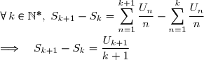
![T_k=\displaystyle\sum_{n=1}^k\dfrac{1}{n(n+1)} \\\overset{ { \white{ . } } } { \phantom{T_k}=\displaystyle\sum_{n=1}^k\dfrac{(n+1)-n}{n(n+1)} } \\\overset{ { \white{ . } } } { \phantom{T_k}=\displaystyle\sum_{n=1}^k\left[\dfrac{n+1}{n(n+1)}-\dfrac{n}{n(n+1)} \right]} \\\overset{ { \white{ . } } } { \phantom{T_k}=\displaystyle\sum_{n=1}^k\left[\dfrac{1}{n}-\dfrac{1}{n+1} \right]}](https://latex.ilemaths.net/latex-0.tex?T_k=\displaystyle\sum_{n=1}^k\dfrac{1}{n(n+1)} \\\overset{ { \white{ . } } } { \phantom{T_k}=\displaystyle\sum_{n=1}^k\dfrac{(n+1)-n}{n(n+1)} } \\\overset{ { \white{ . } } } { \phantom{T_k}=\displaystyle\sum_{n=1}^k\left[\dfrac{n+1}{n(n+1)}-\dfrac{n}{n(n+1)} \right]} \\\overset{ { \white{ . } } } { \phantom{T_k}=\displaystyle\sum_{n=1}^k\left[\dfrac{1}{n}-\dfrac{1}{n+1} \right]})
+\left(\dfrac{1}{2}-\dfrac{1}{3}\right)+\left(\dfrac{1}{3}-\dfrac{1}{4}\right)+\cdots+\left(\dfrac{1}{k-1}-\dfrac{1}{k}\right)+\left(\dfrac{1}{k}-\dfrac{1}{k+1}\right)} \\\overset{ { \white{ . } } } { \phantom{T_k}=\left(1-\cancel{\dfrac{1}{2}}\right)+\left(\cancel{\dfrac{1}{2}}-\cancel{\dfrac{1}{3}}\right)+\left(\cancel{\dfrac{1}{3}}-\cancel{\dfrac{1}{4}}\right)+\cdots+\left(\cancel{\dfrac{1}{k-1}}-\cancel{\dfrac{1}{k}}\right)+\left(\cancel{\dfrac{1}{k}}-\dfrac{1}{k+1}\right)} \\\overset{ { \white{ . } } } { \phantom{T_k}=1-\dfrac{1}{k+1}})

} \\\overset{ { \white{ . } } } { \phantom{WWWWw}\quad\Longrightarrow\quad \displaystyle\sum_{n=1}^k\dfrac{U_n}{n}\le\displaystyle\sum_{n=1}^k\dfrac{\text e^{\frac 3 2}}{n(n+1)} } \\\overset{ { \white{ . } } } { \phantom{WWWWw}\quad\Longrightarrow\quad S_k\le\text e^{\frac 3 2}\displaystyle\sum_{n=1}^k\dfrac{1}{n(n+1)} } \\\overset{ { \white{ . } } } { \phantom{WWWWw}\quad\Longrightarrow\quad S_k\le\text e^{\frac 3 2}T_k })
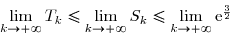
 } \\\\\text{Or }\;1-\dfrac{1}{k+1}\le1\quad\Longrightarrow\quad \text e^{\frac 3 2}\left(1-\dfrac{1}{k+1}\right)\le \text e^{\frac 3 2})
_{k\ge1} }) est convergente vers un réel
est convergente vers un réel 
\\\overset{ { \white{ . } } } { k+1>0 \quad(\text{car }k\in\N^*)\phantom{WWw} } \end{matrix}\right. \quad\Longrightarrow\quad\dfrac{U_{k+1}}{k+1}\ge0)


}\le \dfrac{U_n}{n} \\\overset{ { \white{ . } } } { \phantom{WWWWWWWWw} \quad\Longrightarrow\quad \displaystyle\sum_{n=1}^{k}\dfrac{1}{n(n+1)}\le \displaystyle\sum_{n=1}^{k} \dfrac{U_n}{n} } \\\overset{ { \white{ + } } } { \phantom{WWWWWWWWw} \quad\Longrightarrow\quad T_k\le S_k } \\\\\text{Or }\;S_k\le\text e^{\frac 3 2}\quad(\text{voir 4. b)} \\\\\text{D'où }\;\boxed{\forall\,k\in\N^*,\;T_k\le S_k\le\text e^{\frac 3 2}})
=1 \\\overset{ { \white{ . } } } {\lim\limits_{k\to+\infty}\;\text e^{\frac 3 2}=\text e^{\frac 3 2} }\phantom{xwWWWWWWWx}\end{matrix}\right. )
 , soit
  Publié par malou
le
Publié par malou
le
 Voir la correction
 forum de terminale