1. b) Soit un nombre réel x 0.
D'après la question précédente, nous savons que
Dès lors,
Par conséquent, nous avons montré que :
2. Soit g la fonction numérique de la variable réelle x définie sur ]0 ; +[ par :
Nous devons montrer que :
Par la question précédente, nous savons que :
Dès lors, en divisant les trois membres des inégalités par x ( 0), nous obtenons que pour tout x ]0 ; +[,
Selon le théorème d'encadrement (théorème des gendarmes), nous en déduisons que
Partie II
Soit f la fonction numérique de la variable réelle x définie sur ]0 ; +[ par :
1. Calculons
Nous en déduisons que , soit que
Graphiquement, ce résultat signifie que la courbe C admet une asymptote horizontale d'équation y = 0 au voisinage de +.
2. a) Montrons que la fonction f est continue à droite en 0.
D'une part,
D'autre part,
Dès lors, soit
Par conséquent, la fonction f est continue à droite en 0 car
2. b) Pour tout x ]0 ; +[,
2. c) Nous devons en déduire que f est dérivable à droite de 0 et déterminer
Par conséquent, la fonction f est dérivable à droite de 0 et
3. Montrons que f est dérivable sur ]0 ; +[.
Par définition de f , nous savons que pour tout x ]0 ; +[,
La fonction g est un quotient de deux fonctions dérivables sur ]0 ; +[ avec x 0.
La fonction est dérivable sur ]0 ; +[ comme étant la composée de deux fonctions dérivables.
Il s'ensuit que la fonction f est dérivable sur ]0 ; +[.
De plus, pour tout x ]0 ; +[,
4. a) Nous avons montré dans la Partie I, question 1. b), que pour tout x ]0 ; +[,
Dès lors, pour tout x > 0,
Or
Montrons que pour tout x > 0, nous obtenons
D'où
Dès lors, les "inégalités (1)" peuvent être complétées comme suit :
Par conséquent,
4. b) Puisque l'exponentielle est strictement positive sur , nous avons :
Nous obtenons alors, ,
soit
5. a) En nous basant sur la question précédente, nous pouvons dresser le tableau de variations de f .
5. b) Courbe C et la demi-tangente à droite au point de C de coordonnées (0 ; 1) dont le coefficient directeur vaut
Partie III
1. Montrons que l'équation admet une unique solution dans ]0 ; +[.
Soit la fonction h définie dans ]0 ; +[ par
Notons que
La fonction h est continue sur l'intervalle ]0 ; +[ (somme de deux fonctions continues sur cet intervalle).
La fonction h est strictement décroissante sur l'intervalle ]0 ; +[ (somme de deux fonctions strictement décroissantes sur cet intervalle).
Selon le corollaire du théorème des valeurs intermédiaires, l'équation admet une unique solution dans ]0 ; +[ .
Par conséquent, l'équation admet une unique solution dans ]0 ; +[, soit
2. Soit et la suite numérique définie par :
2. a) Démontrons par récurrence que pour tout entier naturel n ,
Initialisation : Montrons que la propriété est vraie pour n = 0, soit que
C'est une évidence car
Donc l'initialisation est vraie.
Hérédité : Montrons que si pour un nombre naturel n fixé, la propriété est vraie au rang n , alors elle est encore vraie au rang (n +1).
Montrons donc que si pour un nombre naturel n fixé, , alors
En effet, nous savons par la question 5a - Partie II que
Or par hypothèse,
Il s'ensuit que
Par conséquent,
L'hérédité est vraie.
Puisque l'initialisation et l'hérédité sont vraies, nous avons montré par récurrence que
2. b) Nous devons montrer que :
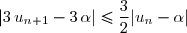
La fonction f est continue et dérivable sur l'intervalle [0 ; +[.
Nous avons montré dans la Partie II - question 4. b) que et par suite,
D'après l'inégalité des accroissements finis sur l'intervalle [0 ; +[, nous obtenons :
Or et
Dès lors,
Il s'ensuit que , soit que
Par conséquent,
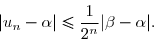
2. c) Démontrons par récurrence que pour tout entier naturel n ,
Initialisation : Montrons que la propriété est vraie pour n = 0, soit que
C'est une évidence car
Donc l'initialisation est vraie.
Hérédité : Montrons que si pour un nombre naturel n fixé, la propriété est vraie au rang n , alors elle est encore vraie au rang (n +1).
Montrons donc que si pour un nombre naturel n fixé, , alors
En effet, nous savons par la question précédente que
Or par hypothèse,
Il s'ensuit que
Par conséquent,
L'hérédité est vraie.
Puisque l'initialisation et l'hérédité sont vraies, nous avons montré par récurrence que
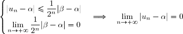
2. d) Montrons que la suite converge vers .
Nous avons montré dans l'exercice précédent que
Donc
Par conséquent,
2,25 points
exercice 2
On considère la fonction numérique : et soit () sa courbe représentative dans un repère orthonormé
Pour tout et pour tout on note le point de la courbe () de coordonnées
1. a) Nous devons montrer que : tel que :
La fonction est continue sur et dérivable sur .
D'après le théorème des accroissements finis, nous déduisons que :
Or
Par conséquent, tel que
1. b) Nous devons montrer que :
Par conséquent,
1. c) Nous avons montré que :
2. Soit la suite numérique définie par :
2. a) Soit
Nous avons montré que
Dès lors,
Changeons les indices dans l'écriture
Soit
Dans ce cas,
Par conséquent,
2. b) Soit la fonction f définie sur [0 ; 1] par
La fonction f est continue sur [0 ; 1].
Rappelons le corollaire du théorème sur les sommes de Riemann.
Soit f une fonction continue sur [a ; b ] (a < b ).
Pour tout , on pose :
Alors les suites et convergent et
Appliquons ce corollaire lorsque a = 0 et b = 1.
Nous obtenons :
De plus,
Dès lors,
Par conséquent,
3,5 points
exercice 3
On considère le nombre complexe :
1. a) Nous devons écrire sous forme exponentielle les nombres complexes : et
Écrivons d'abord sous forme trigonométrique, soit sous la forme
Nous savons que
Nous obtenons ainsi :
Nous en déduisons que la forme trigonométrique de est :
Par conséquent, la forme exponentielle de est :
Écrivons sous forme trigonométrique, soit sous la forme
Nous savons que
Nous obtenons ainsi :
Nous en déduisons que la forme trigonométrique de est :
Par conséquent, la forme exponentielle de est :
1. b) Nous devons montrer que :
1. c) A l'aide de la question précédente, nous obtenons :
Par identification, nous en déduisons que :
Dès lors,
1. d) A l'aide de la question précédente, nous obtenons :
2. On considère les suites et définies par :
et
2. a) Démontrons par récurrence que pour tout entier naturel n ,
Initialisation : Montrons que la propriété est vraie pour n = 0, soit que
C'est une évidence car
Donc l'initialisation est vraie.
Hérédité : Montrons que si pour un nombre naturel n fixé, la propriété est vraie au rang n , alors elle est encore vraie au rang (n +1).
Montrons donc que si pour un nombre naturel n fixé, , alors
En effet,
L'hérédité est vraie.
Puisque l'initialisation et l'hérédité sont vraies, nous avons montré par récurrence que
2. b) Nous en déduisons que pour tout entier naturel n ,
Par identification, nous en déduisons que :
3. Le plan complexe est rapporté à un repère orthonormé direct
Pour tout entier naturel n , on note le point d'affixe
3. a) Nous devons déterminer les entiers n pour lesquels les points et sont alignés.
Les points et sont alignés
Puisque n est un nombre entier naturel, nous avons :
Par conséquent, les points et sont alignés si et seulement si n est multiple de 12.
3. b) Nous devons montrer que pour tout entier n , le triangle OAnAn+1 est rectangle en An .
Montrons d'abord que les trois points et sont distincts deux à deux.
Nous savons que les affixes des points et sont respectivement et
Donc les trois points et forment un triangle.
Montrons ensuite que le triangle OAnAn+1 est rectangle en An .
Le triangle OAnAn+1 est rectangle en An
Par conséquent, le triangle OAnAn+1 est rectangle en An .
3 points
exercice 4
Soit pun nombre premier impair. On considère dans l'équation
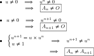
1. a) Montrons que
Puisque p est un nombre premier impair, nous déduisons que
En appliquant le petit théorème de Fermat, nous savons que si p est un nombre premier et si , alors
1. b) Remarques :
et p étant un nombre premier impair donc positif, (p -1) est un nombre pair positif, ce qui implique que
Dès lors,
2. Soit x une solution de l'équation (E ).
2. a) Montrons que p et x sont premiers entre eux.
Nous allons utiliser une propriété des nombres premiers : si un nombre premier ne divise pas un entier, il est premier avec lui.
Montrons alors que le nombre premier p ne divise pas x .
Par l'absurde, supposons que p divise x .
Puisque x une solution de l'équation (E ), nous savons que , soit que .
Donc
Il s'ensuit que :
Ce qui est absurde car p est un nombre premier impair et est donc supérieur ou égal à 3.
D'où la supposition "p divise x " est absurde.
Par conséquent, le nombre premier ne divise pas x .
En utilisant la propriété des nombres premiers rappelée ci-dessus, nous en déduisons que p et x sont premiers entre eux, soit .
2. b) Montrons que :
D'une part, nous savons que p est premier et que
D'après le petit théorème de Fermat, nous déduisons que
D'autre part, x est une solution de l'équation (E ), soit .
Nous avons montré dans les remarques que
Dès lors,
.
Par la transitivité de la congruence modulo p , nous obtenons :
3. Montrons que
Or p ne divise pas k car
D'où, en utilisant la propriété des nombres premiers rappelée dans la question 2. a), nous en déduisons que
En résumé, nous savons que p divise le produit et que p est premier avec k .
Donc, par le théorème de Gauss, p divise
4. a) Montrons que :
Par conséquent,
4. b) On admet que
Nous devons montrer que et que
Nous savons que :
En identifiant les parties réelles, nous obtenons :
Nous en déduisons que
De plus, nous avons montré dans la question 3. que
Autrement dit, , soit
Dès lors,
Puisque nous en déduisons que
5. Nous devons en déduire que si , alors l'équation n'a pas de solution dans
Supposons par l'absurde que x est une solution de l'équation
Dans ce cas, nous avons montré à la question 4. b) que
Dès lors, nous obtenons :
Or nous avons montré dans la question 2. b) que
Nous en déduisons que :
Nous venons de montrer que si x est une solution de l'équation , alors p divise 2, ce qui est impossible, car p étant un nombre premier impair, il est strictement supérieur à 2.
Par conséquent, si , alors l'équation n'a pas de solution dans
3,5 points
exercice 5
On rappelle que est un anneau non commutatif de zéro la matrice et d'unité la matrice , et que est un espace vectoriel réel.
On considère l'ensemble
Partie I
1. Montrons que est un sous-groupe de
Nous savons que est un groupe car est un espace vectoriel.
Pour montrer que est un sous-groupe de , il suffit de montrer que la partie de comprend l'élément neutre du groupe et que
Par conséquent, est un sous-groupe de
2. Montrons que est un sous-espace vectoriel de
En effet,
Par conséquent, est un sous-espace vectoriel de
3. b) Nous devons montrer que est un anneau commutatif et unitaire.
Montrons que est un sous-anneau de .
car
car est un groupe (voir question 1).
car cette propriété a été démontrée dans (voir question 3. a).
D'où est un sous-anneau de .
Par conséquent, est un anneau
Montrons que la loi est commutative dans .
En effet,
Par conséquent, est un anneau commutatif.
Puisque nous en déduisons que est un anneau commutatif et unitaire.
4. a) En utilisant la question 3. a), nous obtenons :
4. b) Nous avons montré que
Or et
Il s'ensuit que l'anneau n'est pas intègre car et sont des diviseurs de zéro.
Par conséquent, étant donné qu'un corps est un anneau intègre, nous en déduisons que n'est pas un corps.
Partie II
Soient et
1. Nous devons montrer que :
Montrons que
En effet,
Supposons que :
Dans ce cas, nous obtenons : , ce qui est impossible puisque et
Donc
De plus,
D'où,
Montrons que C'est évident car
Par conséquent,
2. Nous devons montrer que est un sous-groupe de
Nous savons que
Pour montrer que est un sous-groupe de , il suffit de montrer que et que
car
De plus,
D'où
Par conséquent, est un sous-groupe de
3. Soit l'application définie de vers par :
3. a) Vérifions que
3. b) Nous devons montrer que est un homomorphisme de vers
Par conséquent, est un homomorphisme de vers
3. c) Montrons que est un groupe commutatif.
Nous avons montré dans la question 2 que est un sous-groupe de
Donc est un groupe commutatif car est un groupe commutatif.
Or l'image d'un groupe commutatif par un homomorphisme est un groupe commutatif.
Il s'ensuit que est un groupe commutatif.
Puisque nous déduisons que est un groupe commutatif.
4. Nous devons montrer que est un corps commutatif.
Montrons que est un groupe commutatif. Pour ce faire, montrons que est un sous-groupe commutatif de
est une partie non vide de car En vertu de la question 1 - Partie I, nous obtenons :
Dès lors, est un sous-groupe commutatif de
Par conséquent, est un groupe commutatif.
Nous savons que est un groupe commutatif (voir question 3. c).
La multiplication est distributive par rapport à l'addition dans car la multiplication est distributive par rapport à l'addition dans
Par conséquent, est un corps commutatif.
Publié par malou
le
ceci n'est qu'un extrait
Pour visualiser la totalité des cours vous devez vous inscrire / connecter (GRATUIT) Inscription Gratuitese connecter
Merci à Hiphigenie / malou pour avoir contribué à l'élaboration de cette fiche
Désolé, votre version d'Internet Explorer est plus que périmée ! Merci de le mettre à jour ou de télécharger Firefox ou Google Chrome pour utiliser le site. Votre ordinateur vous remerciera !
^2}\le\dfrac{1}{1+t}\le\dfrac 1 2\left(1+\dfrac{1}{(1+t)^2}\right) \,. })
^2}-\dfrac{1}{1+t}=\dfrac{4(1+t)-(2+t)^2}{(2+t)^2(1+t)} \\ \overset{ { \white{ . } } } { \phantom{WWWWWWWWWWWWWW}= \dfrac{4+4t-4-4t-t^2}{(2+t)^2(1+t)} } \\ \overset{ { \white{ . } } } { \phantom{WWWWWWWWWWWWWW}= \dfrac{-t^2}{(2+t)^2(1+t)} })
^2>0\\1+t>0\end{matrix}\right.\quad\Longrightarrow\quad \dfrac{-t^2}{(2+t)^2(1+t)}\le0 \\\phantom{WWWWWWWWWWWWW}\quad\Longrightarrow\quad \dfrac{4}{(2+t)^2}-\dfrac{1}{1+t}\le0)
^2}\le\dfrac{1}{1+t}})
^2}\right)=\dfrac{1}{1+t}-\dfrac 1 2-\dfrac{1}{2(1+t)^2} \\ \overset{ { \white{ . } } } { \phantom{WWWWWWWWWWWWWWWwWW}= \dfrac{2(1+t)-(1+t)^2-1}{2(1+t)^2} } \\ \overset{ { \white{ . } } } { \phantom{WWWWWWWWWWWWWWWwWW}= \dfrac{2+2t-1-2t-t^2-1}{2(1+t)^2} } \\ \overset{ { \phantom{ . } } } { \phantom{WWWWWWWWWWWWWWWwWW}= \dfrac{-t^2}{2(1+t)^2} } )
^2>0\end{matrix}\right.\quad\Longrightarrow\quad \dfrac{-t^2}{2(1+t)^2}\le0 \\\overset{ { \white{ . } } } { \phantom{WWWWWWWWWWWWwW}\quad\Longrightarrow\quad \dfrac{1}{1+t}-\dfrac 1 2\left(1+\dfrac{1}{(1+t)^2}\right)\le0})
^2}\right) })
^2}\le\dfrac{1}{1+t}\le\dfrac 1 2\left(1+\dfrac{1}{(1+t)^2}\right) } \,. })
 0.
0.![\overset{ { \white{ . } } } { \forall\,t\in[0\;;\;x],\;\dfrac{4}{(2+t)^2}\le\dfrac{1}{1+t}\le\dfrac 1 2\left(1+\dfrac{1}{(1+t)^2}\right) \,. }](https://latex.ilemaths.net/latex-0.tex?\overset{ { \white{ . } } } { \forall\,t\in[0\;;\;x],\;\dfrac{4}{(2+t)^2}\le\dfrac{1}{1+t}\le\dfrac 1 2\left(1+\dfrac{1}{(1+t)^2}\right) \,. })
![\displaystyle\int_0^{x}\dfrac{4}{(2+t)^2}\text{ d}t\le\displaystyle\int_0^{x}\dfrac{1}{1+t}\text{ d}t\le\displaystyle\int_0^{x}\dfrac 1 2\left(1+\dfrac{1}{(1+t)^2}\right)\text{ d}t \\ \\ \quad\Longrightarrow\quad4\left[\dfrac{-1}{2+t}\right]_0^x\le\left[\overset{{\white{\frac{}{}}}}{\ln(1+t)}\right]_0^x\le\dfrac 1 2 \left[t-\dfrac{1}{1+t}\right]_0^x \\ \\ \quad\Longrightarrow\quad4\left(\dfrac{-1}{2+x}-\dfrac{-1}{2+0}\right)\le\ln(1+x)-\ln(1+0)\le\dfrac 1 2 \left[\left(x-\dfrac{1}{1+x}\right)-\left(0-\dfrac{1}{1+0}\right)\right] \\ \\ \quad\Longrightarrow\quad4\left(\dfrac{-1}{2+x}+\dfrac{1}{2}\right)\le\ln(1+x)-0\le\dfrac 1 2 \left(x-\dfrac{1}{1+x}+1\right)](https://latex.ilemaths.net/latex-0.tex?\displaystyle\int_0^{x}\dfrac{4}{(2+t)^2}\text{ d}t\le\displaystyle\int_0^{x}\dfrac{1}{1+t}\text{ d}t\le\displaystyle\int_0^{x}\dfrac 1 2\left(1+\dfrac{1}{(1+t)^2}\right)\text{ d}t \\ \\ \quad\Longrightarrow\quad4\left[\dfrac{-1}{2+t}\right]_0^x\le\left[\overset{{\white{\frac{}{}}}}{\ln(1+t)}\right]_0^x\le\dfrac 1 2 \left[t-\dfrac{1}{1+t}\right]_0^x \\ \\ \quad\Longrightarrow\quad4\left(\dfrac{-1}{2+x}-\dfrac{-1}{2+0}\right)\le\ln(1+x)-\ln(1+0)\le\dfrac 1 2 \left[\left(x-\dfrac{1}{1+x}\right)-\left(0-\dfrac{1}{1+0}\right)\right] \\ \\ \quad\Longrightarrow\quad4\left(\dfrac{-1}{2+x}+\dfrac{1}{2}\right)\le\ln(1+x)-0\le\dfrac 1 2 \left(x-\dfrac{1}{1+x}+1\right))
}\right)\le\ln(1+x)\le\dfrac 1 2 \left(\dfrac{x+x^2-1+1+x}{1+x}\right) \\ \\ \quad\Longrightarrow\quad4\left(\dfrac{x}{2(2+x)}\right)\le\ln(1+x)\le\dfrac 1 2 \left(\dfrac{x^2+2x}{1+x}\right) \\ \\ \quad\Longrightarrow\quad\dfrac{2x}{2+x}\le\ln(1+x)\le\dfrac 1 2 \left(\dfrac{x^2+2x}{1+x}\right))
\le\dfrac 1 2 \left(\dfrac{x^2+2x}{1+x}\right) } \,. })
 [ par :
 =\dfrac{\ln(1+x)}{x}\,.})
-1}{x}=\dfrac{-1}{2}\,.})
![\overset{ { \white{ . } } } { \forall\,x\in\;]0\;;\;+\infty[,\; \dfrac{2x}{2+x}\le\ln(1+x)\le\dfrac 1 2 \left(\dfrac{x(x+2)}{1+x}\right) }](https://latex.ilemaths.net/latex-0.tex?\overset{ { \white{ . } } } { \forall\,x\in\;]0\;;\;+\infty[,\; \dfrac{2x}{2+x}\le\ln(1+x)\le\dfrac 1 2 \left(\dfrac{x(x+2)}{1+x}\right) })
 0), nous obtenons que pour tout x
  ]0 ; +
}{x}\le\dfrac 1 2 \left(\dfrac{x+2}{1+x}\right)\quad\Longrightarrow\quad\dfrac{2}{2+x}\le g(x)\le\dfrac{x+2}{2(1+x)} \\ \overset{ { \white{ . } } } { \phantom{WWWWWWWWWWWWW}\quad\Longrightarrow\quad\dfrac{2}{2+x}-1\le g(x)-1\le\dfrac{x+2}{2(1+x)}-1 } \\ \overset{ { \white{ . } } } { \phantom{WWWWWWWWWWWWW}\quad\Longrightarrow\quad\dfrac{2-2-x}{2+x}\le g(x)-1\le\dfrac{x+2-2-2x}{2(1+x)} } \\ \overset{ { \white{ . } } } { \phantom{WWWWWWWWWWWWW}\quad\Longrightarrow\quad\dfrac{-x}{2+x}\le g(x)-1\le\dfrac{-x}{2(1+x)} })
-1}{x}\le\dfrac{-1}{2(1+x)} } \\\\\text{Or }\;\left\lbrace\begin{matrix}\underset{x>0}{\underset{x\to0}{\lim}}\;\dfrac{-1}{2+x}=-\dfrac 1 2 \\\overset{ { \white{ . } } } { \underset{x>0}{\underset{x\to0}{\lim}}\;\dfrac{-1}{2(1+x)}=-\dfrac 1 2 }\end{matrix}\right. )
-1}{x}=-\dfrac 12 }\,.)
![\left\lbrace\begin{matrix}f(0)=1\phantom{WWWWWWWWWWx}\\f(x)=g(x)\,\text e^{-x}\quad(\forall\,x\in\;]0\;;\;+\infty\,[)\end{matrix}\right.](https://latex.ilemaths.net/latex-0.tex?\left\lbrace\begin{matrix}f(0)=1\phantom{WWWWWWWWWWx}\\f(x)=g(x)\,\text e^{-x}\quad(\forall\,x\in\;]0\;;\;+\infty\,[)\end{matrix}\right.)
. })
=\lim\limits_{x\to+\infty}g(x)\,\text e^{-x} \\ \overset{ { \white{ . } } } { \phantom{WWWvW}= \lim\limits_{x\to+\infty}\dfrac{\ln(1+x)}{x}\,\text e^{-x}} \\ \overset{ { \white{ . } } } { \phantom{WWWvW}= \lim\limits_{x\to+\infty}\dfrac{\ln(1+x)}{1+x}\times\dfrac{1+x}{x}\times\text e^{-x}})
}{1+x}=\lim\limits_{X\to+\infty}\dfrac{\ln(X)}{X}\quad\text{avec }X=1+x\\\overset{ { \white{ . } } } { \phantom{WWWWi}=0\quad\text{croissances comparées }}\\ \\\lim\limits_{x\to+\infty}\dfrac{1+x}{x}=\lim\limits_{x\to+\infty}\dfrac{x}{x}=1 \phantom{WWWWWWWWW}\\ \\\lim\limits_{x\to+\infty}\text e^{-x}\underset{(X=-x)}{=}\;\lim\limits_{X\to-\infty}\text e^{X}=0\phantom{WWWWWWW}\end{matrix}\right.)
=0\times1\times0 }) , soit que
, soit que =0}\,. })
=1}}.)
= \underset{x>0}{\underset{x\to0}{\lim}}\;\dfrac{\ln(1+x)}{x}\,\text e^{-x}\,.)
}{x}=\underset{x>0}{\underset{x\to0}{\lim}}\;\dfrac{\ln(1+x)-\ln(1+0)}{x-0} \\ \\ \overset{ { \white{ . } } } { \phantom{WWWWiWWW}=h'(0)\quad\text{avec }h(x)=\ln(1+x) } \\ \overset{ { \white{ . } } } { \phantom{WWWWiWWW}=1\quad\text{car }h'(x)=\dfrac{1}{1+x}\Longrightarrow\quad h'(0)=\dfrac{1}{1+0}=1 } \\ \\\text{D'où }\;\boxed{\underset{x>0}{\underset{x\to0}{\lim}}\;\dfrac{\ln(1+x)}{x}=1 })

}{x}\,\text e^{-x}=1\times 1 = 1, }) soit
soit = 1}}. })
= f(0). })
![\left(\dfrac{\text e^{-x}-1}{x}\right)g(x)+\left(\dfrac{g(x)-1}{x}\right)=\dfrac{(\text e^{-x}-1)g(x)+g(x)-1}{x} \\ \overset{ { \white{ . } } } { \phantom{WWWWWWWWWxWWW}= \dfrac{\text e^{-x}g(x)-g(x)+g(x)-1}{x}} \\ \overset{ { \white{ . } } } { \phantom{WWWWWWWWWxWWW}= \dfrac{\text e^{-x}g(x)-1}{x}} \\ \overset{ { \white{ . } } } { \phantom{WWWWWWWWWxWWW}= \dfrac{f(x)-1}{x}} \\ \\ \Longrightarrow\quad\boxed{\forall\,x\in\,]0\;;\;+\infty[,\; \dfrac{f(x)-1}{x}=\left(\dfrac{\text e^{-x}-1}{x}\right)g(x)+\left(\dfrac{g(x)-1}{x}\right) }](https://latex.ilemaths.net/latex-0.tex?\left(\dfrac{\text e^{-x}-1}{x}\right)g(x)+\left(\dfrac{g(x)-1}{x}\right)=\dfrac{(\text e^{-x}-1)g(x)+g(x)-1}{x} \\ \overset{ { \white{ . } } } { \phantom{WWWWWWWWWxWWW}= \dfrac{\text e^{-x}g(x)-g(x)+g(x)-1}{x}} \\ \overset{ { \white{ . } } } { \phantom{WWWWWWWWWxWWW}= \dfrac{\text e^{-x}g(x)-1}{x}} \\ \overset{ { \white{ . } } } { \phantom{WWWWWWWWWxWWW}= \dfrac{f(x)-1}{x}} \\ \\ \Longrightarrow\quad\boxed{\forall\,x\in\,]0\;;\;+\infty[,\; \dfrac{f(x)-1}{x}=\left(\dfrac{\text e^{-x}-1}{x}\right)g(x)+\left(\dfrac{g(x)-1}{x}\right) })
. })
-f(0)}{x-0}=\underset{x>0}{\underset{x\to0}{\lim}}\;\dfrac{f(x)-1}{x} \\ \overset{ { \white{ . } } } { \phantom{WWWWWxW}= \underset{x>0}{\underset{x\to0}{\lim}}\;\left(\dfrac{\text e^{-x}-1}{x}\right)g(x)+\left(\dfrac{g(x)-1}{x}\right) })
= \underset{x>0}{\underset{x\to0}{\lim}}\;\left(\dfrac{\text e^{-x}-\text e^0}{x-0}\right) \\ \overset{ { \white{ . } } } { \phantom{WWWWWWWWWW}= k'(0)\quad\text{avec }k(x)=\text e^{-x} } \\ \overset{ { \white{ . } } } { \phantom{WWWWWWWWWW}= -1\quad\text{car }k'(x)=-\text e^{-x}\Longrightarrow\quad k'(0)=-\text e^{0}=-1 } \\\\\phantom{WWWW}\text{D'où }\;\boxed{\underset{x>0}{\underset{x\to0}{\lim}}\;\left(\dfrac{\text e^{-x}-1}{x}\right)=-1 })
=\underset{x>0}{\underset{x\to0}{\lim}}\;\dfrac{\ln(1+x)}{x}=1\quad(\text{voir Partie II - 2. a)}\quad\Longrightarrow\;\boxed{\underset{x>0}{\underset{x\to0}{\lim}}\;g(x)=1 } \\\\\bullet\quad\boxed{\underset{x>0}{\underset{x\to0}{\lim}}\;\left(\dfrac{g(x)-1}{x}\right)=-\dfrac 1 2 }\quad(\text{voir Partie I - 2.)} \\ \\ \\ \text{D'où }\;\underset{x>0}{\underset{x\to0}{\lim}}\;\dfrac{f(x)-f(0)}{x-0}=(-1)\times1+\left(-\dfrac 1 2\right)=-1-\dfrac 1 2 \\ \quad\Longrightarrow\boxed{\underset{x>0}{\underset{x\to0}{\lim}}\;\dfrac{f(x)-f(0)}{x-0}=-\dfrac 3 2 \in\R})
=-\dfrac 3 2 . })
=g(x)\,\text e^{-x}.)
 est dérivable sur ]0 ; +
=\left(\dfrac{\ln(1+x)}{x}\,\text e^{-x}\right)' \\ \overset{ { \white{ . } } } { \phantom{f'(x)}=\left(\dfrac{\ln(1+x)}{x}\right)' \times\text e^{-x}+\dfrac{\ln(1+x)}{x}\times(\text e^{-x})'} \\ \overset{ { \white{ . } } } { \phantom{f'(x)}=\dfrac{(\ln(1+x))'\times x-\ln(1+x)\times x'}{x^2}}\times\text e^{-x}+\dfrac{\ln(1+x)}{x}\times(-\text e^{-x}) \\ \overset{ { \white{ . } } } { \phantom{f'(x)}=\dfrac{\dfrac{1}{1+x}\times x-\ln(1+x)\times 1}{x^2}}\times\text e^{-x}-\dfrac{\ln(1+x)}{x}\times\text e^{-x})

}=\dfrac{\dfrac{x}{1+x}-\ln(1+x)}{x^2} }\times\text e^{-x}-\dfrac{\ln(1+x)}{x}\times\text e^{-x} \\ \overset{ { \white{ . } } } { \phantom{f'(x)}=\left(\dfrac{\dfrac{x}{1+x}-\ln(1+x)}{x^2} -\dfrac{\ln(1+x)}{x}\right)\times\text e^{-x}} \\ \overset{ { \white{ . } } } { \phantom{f'(x)}=\left(\dfrac{\dfrac{x-(1+x)\ln(1+x)}{1+x}}{x^2} -\dfrac{\ln(1+x)}{x}\right)\times\text e^{-x}})
}=\left(\dfrac{x-(1+x)\ln(1+x)}{x^2(1+x)} -\dfrac{\ln(1+x)}{x}\right)\times\text e^{-x}} \\ \overset{ { \white{ . } } } { \phantom{f'(x)}=\left(\dfrac{x-(1+x)\ln(1+x)}{x^2(1+x)} -\dfrac{x(1+x)\ln(1+x)}{x^2(1+x)}\right)\times\text e^{-x}} \\ \overset{ { \white{ . } } } { \phantom{f'(x)}=\dfrac{x-(1+x)\ln(1+x)-x(1+x)\ln(1+x)}{x^2(1+x)} \times\text e^{-x}})
![\\ \overset{ { \white{ . } } } { \phantom{f'(x)}=\dfrac{x-(1+x)\ln(1+x)[1+x]}{x^2(1+x)} \,\text e^{-x}} \\ \overset{ { \white{ . } } } { \phantom{f'(x)}=\dfrac{x-(1+x)^2\ln(1+x)}{x^2(1+x)} \,\text e^{-x}} \\ \\ \Longrightarrow\quad\boxed{\forall\,x\in\,]\,0\;;\;+\infty\,[,\;f'(x)=\dfrac{x-(1+x)^2\ln(1+x)}{x^2(1+x)} \,\text e^{-x}}](https://latex.ilemaths.net/latex-0.tex?\\ \overset{ { \white{ . } } } { \phantom{f'(x)}=\dfrac{x-(1+x)\ln(1+x)[1+x]}{x^2(1+x)} \,\text e^{-x}} \\ \overset{ { \white{ . } } } { \phantom{f'(x)}=\dfrac{x-(1+x)^2\ln(1+x)}{x^2(1+x)} \,\text e^{-x}} \\ \\ \Longrightarrow\quad\boxed{\forall\,x\in\,]\,0\;;\;+\infty\,[,\;f'(x)=\dfrac{x-(1+x)^2\ln(1+x)}{x^2(1+x)} \,\text e^{-x}})
\le\dfrac 1 2 \left(\dfrac{x^2+2x}{1+x}\right) \,. })
^2\times\,}} \dfrac 1 2 \left(\dfrac{x^2+2x}{1+x}\right) \le{\red{-(1+x)^2\times\,}}\ln(1+x)\le{\red{-(1+x)^2\times\,}}\dfrac{2x}{2+x} } \\ \overset{ { \white{ . } } } { -\dfrac 1 2 (1+x)(x^2+2x) \le-(1+x)^2\ln(1+x)\le-(1+2x+x^2)\times\dfrac{2x}{2+x} } \\ \overset{ { \white{ . } } } { -\dfrac 1 2 (x^2+2x+x^3+2x^2) \le-(1+x)^2\ln(1+x)\le-\dfrac{2x+4x^2+2x^3}{2+x} })
^2\ln(1+x)\le x-\dfrac{2x+4x^2+2x^3}{2+x} } \\ \overset{ { \white{ . } } } { \dfrac {2x-x^2-2x-x^3-2x^2}{ 2} \le x-(1+x)^2\ln(1+x)\le \dfrac{2x+x^2-2x-4x^2-2x^3}{2+x} } \\ \overset{ { \white{ . } } } { \dfrac {-x^3-3x^2}{ 2} \le x-(1+x)^2\ln(1+x)\le \dfrac{-2x^3-3x^2}{2+x} } )
}{ 2} \le x-(1+x)^2\ln(1+x)\le \dfrac{-x^2(2x+3)}{2+x} } \\ \overset{ { \white{ . } } } { \dfrac {-x^2(x+3)}{ 2x^2(1+x)} \le\dfrac{ x-(1+x)^2\ln(1+x)}{x^2(1+x)}\le \dfrac{-x^2(2x+3)}{x^2(1+x)(2+x)} }\quad\text{car }x^2(1+x)>0 \\ \overset{ { \white{ . } } } { \dfrac {-(x+3)}{ 2(1+x)} \le\dfrac{ x-(1+x)^2\ln(1+x)}{x^2(1+x)}\le \dfrac{-(2x+3)}{(1+x)(2+x)} }\quad{\red{\text{(inégalités }(1))}})
(2+x)}>0\quad\Longrightarrow\quad\boxed{\dfrac{-(2x+3)}{(1+x)(2+x)}<0} })
}{ 2(1+x)} .)
}{ 2(1+x)} \quad\Longleftrightarrow\quad\dfrac 3 2 >\dfrac {x+3}{ 2(1+x)} \\ \overset{ { \white{ . } } } { \phantom{WWWiWWW} \quad\Longleftrightarrow\quad3 >\dfrac {x+3}{ 1+x} } \\ \overset{ { \white{ . } } } { \phantom{WWWiWWW} \quad\Longleftrightarrow\quad3(1+x) >x+3 } \\ \overset{ { \white{ . } } } { \phantom{WWWiWWW} \quad\Longleftrightarrow\quad3+3x >x+3 })


}{ 2(1+x)} }})
}{ 2(1+x)} \le\dfrac{ x-(1+x)^2\ln(1+x)}{x^2(1+x)}\le \dfrac{-(2x+3)}{(1+x)(2+x)} <0)
![\overset{ { \white{ . } } } { \boxed{\forall\,x\in\,]0\;;\;+\infty\,[,\;-\dfrac 3 2 <\dfrac{ x-(1+x)^2\ln(1+x)}{x^2(1+x)} <0}}](https://latex.ilemaths.net/latex-0.tex?\overset{ { \white{ . } } } { \boxed{\forall\,x\in\,]0\;;\;+\infty\,[,\;-\dfrac 3 2 <\dfrac{ x-(1+x)^2\ln(1+x)}{x^2(1+x)} <0}})
 , nous avons :
 ![\forall\,x\in\,]0\;;\;+\infty\,[,\;-\dfrac 3 2 <\dfrac{ x-(1+x)^2\ln(1+x)}{x^2(1+x)} <0 \\\\ \phantom{XXX}\quad\Longrightarrow\quad -\dfrac 3 2\,\text e^{-x} <\dfrac{ x-(1+x)^2\ln(1+x)}{x^2(1+x)}\,\text e^{-x} <0 \\\\ \phantom{XXX}\quad\Longrightarrow\quad -\dfrac 3 2\,\text e^{-x} <f'(x)<0](https://latex.ilemaths.net/latex-0.tex?\forall\,x\in\,]0\;;\;+\infty\,[,\;-\dfrac 3 2 <\dfrac{ x-(1+x)^2\ln(1+x)}{x^2(1+x)} <0 \\\\ \phantom{XXX}\quad\Longrightarrow\quad -\dfrac 3 2\,\text e^{-x} <\dfrac{ x-(1+x)^2\ln(1+x)}{x^2(1+x)}\,\text e^{-x} <0 \\\\ \phantom{XXX}\quad\Longrightarrow\quad -\dfrac 3 2\,\text e^{-x} <f'(x)<0 )
![\forall\,x\in\,]0\;;\;+\infty\,[,\; -\dfrac 3 2 <-\dfrac 3 2\,\text e^{-x} <f'(x)<0](https://latex.ilemaths.net/latex-0.tex?\forall\,x\in\,]0\;;\;+\infty\,[,\; -\dfrac 3 2 <-\dfrac 3 2\,\text e^{-x} <f'(x)<0 ) ,
,![\boxed{\forall\,x\in\,]0\;;\;+\infty\,[,\; -\dfrac 3 2 <f'(x)<0 }](https://latex.ilemaths.net/latex-0.tex?\boxed{\forall\,x\in\,]0\;;\;+\infty\,[,\; -\dfrac 3 2 <f'(x)<0 })
=1\phantom{W}\\ \\f_d(0)=-\dfrac 3 2<0\end{matrix}\phantom{ WW } \begin{matrix}|\\|\\|\\|\\|\\|\\|\\|\\|\end{matrix}\phantom{ WW }\begin{array} { |c|ccccccc| } \hline &&&&&&&& x &0&&&&&&+\infty\\ &&&&&&& \\ \hline&&&&&&& \\ f'(x)&& - && - & &- &\\&&&&&&&\\ \hline&1&&&&&&\\ f(x)&&\searrow&&\searrow&&\searrow&\\&&&& &&&0\\ \hline \end{array})

=3x }) admet une unique solution
admet une unique solution  dans ]0 ; +
=f(x)-3x .})
=f(x)-3x\quad\Longleftrightarrow\quad h(x)=f(x)+(-3x) .})
![\left\lbrace\begin{matrix}\lim\limits_{ x\to0^+ }h(x)=\lim\limits_{ x\to0^+ }[f(x)-3x]=1-0=1\phantom{ www }\\\lim\limits_{ x\to+\infty }h(x)=\lim\limits_{ x\to+\infty } [f(x)-3x]=0-\infty=-\infty \end{matrix}\right.\quad\Longrightarrow\quad \boxed{ 0\in\,]\,\lim\limits_{ x\to+\infty }h(x)\,;\,\lim\limits_{ x\to0^+ }h(x)\,[ }](https://latex.ilemaths.net/latex-0.tex?\left\lbrace\begin{matrix}\lim\limits_{ x\to0^+ }h(x)=\lim\limits_{ x\to0^+ }[f(x)-3x]=1-0=1\phantom{ www }\\\lim\limits_{ x\to+\infty }h(x)=\lim\limits_{ x\to+\infty } [f(x)-3x]=0-\infty=-\infty \end{matrix}\right.\quad\Longrightarrow\quad \boxed{ 0\in\,]\,\lim\limits_{ x\to+\infty }h(x)\,;\,\lim\limits_{ x\to0^+ }h(x)\,[ })
=0 } }) admet une unique solution
admet une unique solution =3x }) admet une unique solution
admet une unique solution =3\alpha}\, . })
 et
et _{n\in\N} } ) la suite numérique définie par :
la suite numérique définie par : \quad(\forall\,n\in\N) }\end{matrix}\right.} )


 , alors
![\overset{ { \white{ . } } } { \forall\,x\in\;]0\;;\;+\infty\,[,\; f(x)>0. }](https://latex.ilemaths.net/latex-0.tex?\overset{ { \white{ . } } } { \forall\,x\in\;]0\;;\;+\infty\,[,\; f(x)>0. })
![\overset{ { \white{ . } } } { u_n\in\;]0\;;\;+\infty\,[. }](https://latex.ilemaths.net/latex-0.tex?\overset{ { \white{ . } } } { u_n\in\;]0\;;\;+\infty\,[. })
>0. })


![\forall\,x\in\,]0\;;\;+\infty\,[,\; -\dfrac 3 2 <f'(x)<0](https://latex.ilemaths.net/latex-0.tex?\forall\,x\in\,]0\;;\;+\infty\,[,\; -\dfrac 3 2 <f'(x)<0 ) et par suite,
et par suite, |<\dfrac 3 2.)
-f(y)|\le \dfrac 3 2|x-y|.})
 et
et 
-f(\alpha)|\le \dfrac 3 2|u_n-\alpha|\,.)
 , soit que
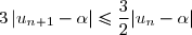

 , alors


^n=0\quad\text{car }0<\dfrac 1 2<1 \\\\\text{D'où }\;\lim\limits_{n\to+\infty}\dfrac{1}{2^n}|\beta-\alpha|=0)
 et soit (
 ) sa courbe représentative dans un repère
 .})
 et pour tout
  on note
  le point de la courbe (
.)
![\overset{ { \white{ . } } } { \forall\,k\in\lbrace0;1;\cdots;(n-1)\rbrace ,\;\exists\,c_k\in\left]\dfrac k n\;;\;\dfrac{k+1}{n}\right[ }](https://latex.ilemaths.net/latex-0.tex?\overset{ { \white{ . } } } { \forall\,k\in\lbrace0;1;\cdots;(n-1)\rbrace ,\;\exists\,c_k\in\left]\dfrac k n\;;\;\dfrac{k+1}{n}\right[ }) tel que :
tel que : 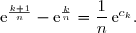
 est continue sur
 ![\left[\dfrac k n\;;\;\dfrac{k+1}{n}\right]](https://latex.ilemaths.net/latex-0.tex?\left[\dfrac k n\;;\;\dfrac{k+1}{n}\right]) et dérivable sur
et dérivable sur ![\left]\dfrac k n\;;\;\dfrac{k+1}{n}\right[](https://latex.ilemaths.net/latex-0.tex?\left]\dfrac k n\;;\;\dfrac{k+1}{n}\right[) .
.![\overset{ { \white{ . } } } { \exists\,c_k\in\left]\dfrac k n\;;\;\dfrac{k+1}{n}\right[:f\left(\dfrac{k+1}{n}\right)-f\left(\dfrac{k}{n}\right)=f'(c_k)\left(\dfrac{k+1}{n}-\dfrac k n\right) }](https://latex.ilemaths.net/latex-0.tex?\overset{ { \white{ . } } } { \exists\,c_k\in\left]\dfrac k n\;;\;\dfrac{k+1}{n}\right[:f\left(\dfrac{k+1}{n}\right)-f\left(\dfrac{k}{n}\right)=f'(c_k)\left(\dfrac{k+1}{n}-\dfrac k n\right) })
=\text e^{\frac k n}\phantom{WWWWWWWWWW}\\\overset{ { \white{ P } } } { f\left(\dfrac{k+1}{n}\right)=\text e^{\frac{k+1}{n}} }\phantom{WWWWWWWW}\\\overset{ { \white{ P } } } { f'(x)=(\text e^x)'=\text e^x\quad\Longrightarrow\quad f'(c_k)=\text e^{c_k} }\\\overset{ { \white{ P } } } { \dfrac{k+1}{n}-\dfrac k n=\dfrac{k+1-k}{n}=\dfrac 1 n }\phantom{WxWWW}\end{matrix}\right.)
\rbrace ;\; M_kM_{k+1}=\dfrac 1 n \sqrt{1+\text e^{2c_k}} })
![\left\lbrace\begin{matrix}M_k\ \left(\dfrac k n\;;\;\text e^{\frac k n}\right)\\ \\ M_{k+1}\ \left(\dfrac {k+1} {n}\;;\;\text e^{\frac {k+1}{n}}\right)\end{matrix}\right.\quad\Longrightarrow\quad\begin{matrix}\\ \\ \\ \\ \\ \\ \\ \\ M_kM_{k+1}=\sqrt{\left(\dfrac{k+1}{n}-\dfrac{k}{n}\right)^2+\left(\text e^{\frac {k+1}{n}}-\text e^{\frac {k}{n}}\right)^2 }\\\overset{ { \white{ . } } } { \phantom{wwwww}=\sqrt{\left(\dfrac{1}{n}\right)^2+\left(\dfrac 1 n \,\text e^{c_k}\right)^2 }\quad(\text{voir 1. a}) }\\ \overset{ { \white{P } } } { \phantom{wwwwwww}=\sqrt{\left(\dfrac{1}{n}\right)^2\,\left[1+\left(\,\text e^{c_k}\right)^2\right] }\phantom{ WWWwWwW } }\\ \overset{ { \white{P } } } { =\dfrac{1}{n}\sqrt{1+\text e^{2c_k}\ }\phantom{ WWWwW }}\end{matrix}](https://latex.ilemaths.net/latex-0.tex?\left\lbrace\begin{matrix}M_k\ \left(\dfrac k n\;;\;\text e^{\frac k n}\right)\\ \\ M_{k+1}\ \left(\dfrac {k+1} {n}\;;\;\text e^{\frac {k+1}{n}}\right)\end{matrix}\right.\quad\Longrightarrow\quad\begin{matrix}\\ \\ \\ \\ \\ \\ \\ \\ M_kM_{k+1}=\sqrt{\left(\dfrac{k+1}{n}-\dfrac{k}{n}\right)^2+\left(\text e^{\frac {k+1}{n}}-\text e^{\frac {k}{n}}\right)^2 }\\\overset{ { \white{ . } } } { \phantom{wwwww}=\sqrt{\left(\dfrac{1}{n}\right)^2+\left(\dfrac 1 n \,\text e^{c_k}\right)^2 }\quad(\text{voir 1. a}) }\\ \overset{ { \white{P } } } { \phantom{wwwwwww}=\sqrt{\left(\dfrac{1}{n}\right)^2\,\left[1+\left(\,\text e^{c_k}\right)^2\right] }\phantom{ WWWwWwW } }\\ \overset{ { \white{P } } } { =\dfrac{1}{n}\sqrt{1+\text e^{2c_k}\ }\phantom{ WWWwW }}\end{matrix})
\rbrace ;\; M_kM_{k+1}=\dfrac 1 n \sqrt{1+\text e^{2c_k}} })
![\text{Or }\;c_k\in\left]\dfrac k n\;;\;\dfrac{k+1}{n}\right[\quad\Longrightarrow\quad c_k\in\left[\dfrac k n\;;\;\dfrac{k+1}{n}\right] \\ \overset{ { \white{ . } } } {\phantom{WWWWWWWWw} \quad\Longrightarrow\quad \dfrac k n\le c_k\le \dfrac{k+1}{n} } \\ \overset{ { \phantom{ . } } } {\phantom{WWWWWWWWw} \quad\Longrightarrow\quad \dfrac {2k}{ n}\le 2c_k\le \dfrac{2(k+1)}{n} } \\ \overset{ { \white{P } } } {\phantom{WWWWWWWWw} \quad\Longrightarrow\quad \text e^{\frac {2k}{ n} }\le \text e^{2c_k}\le \text e^{\frac{2(k+1)}{n}} } \\ \overset{ { \white{P } } } {\phantom{WWWWWWWWw} \quad\Longrightarrow\quad 1+\text e^{\frac {2k}{ n} }\le 1+\text e^{2c_k}\le 1+\text e^{\frac{2(k+1)}{n}} }](https://latex.ilemaths.net/latex-0.tex?\text{Or }\;c_k\in\left]\dfrac k n\;;\;\dfrac{k+1}{n}\right[\quad\Longrightarrow\quad c_k\in\left[\dfrac k n\;;\;\dfrac{k+1}{n}\right] \\ \overset{ { \white{ . } } } {\phantom{WWWWWWWWw} \quad\Longrightarrow\quad \dfrac k n\le c_k\le \dfrac{k+1}{n} } \\ \overset{ { \phantom{ . } } } {\phantom{WWWWWWWWw} \quad\Longrightarrow\quad \dfrac {2k}{ n}\le 2c_k\le \dfrac{2(k+1)}{n} } \\ \overset{ { \white{P } } } {\phantom{WWWWWWWWw} \quad\Longrightarrow\quad \text e^{\frac {2k}{ n} }\le \text e^{2c_k}\le \text e^{\frac{2(k+1)}{n}} } \\ \overset{ { \white{P } } } {\phantom{WWWWWWWWw} \quad\Longrightarrow\quad 1+\text e^{\frac {2k}{ n} }\le 1+\text e^{2c_k}\le 1+\text e^{\frac{2(k+1)}{n}} })
}{n}} } } \\ \overset{ { \white{P } } } {\phantom{WWWWWWWWw} \quad\Longrightarrow\quad \dfrac 1 n\sqrt{ 1+\text e^{\frac {2k}{ n} } }\le \dfrac 1 n\sqrt{ 1+\text e^{2c_k} }\le \dfrac 1 n\sqrt{ 1+\text e^{\frac{2(k+1)}{n}} } } \\\\\text{D'où }\;\boxed{\forall\,k\in\lbrace0;1;\cdots;(n-1)\rbrace ;\;\dfrac 1 n\sqrt{ 1+\text e^{\frac {2k}{ n} } }\le M_kM_{k+1}\le \dfrac 1 n\sqrt{ 1+\text e^{\frac{2(k+1)}{n}} }} )
_{n\in\N^*} }) la suite numérique définie par :
la suite numérique définie par : 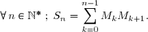

\rbrace ;\;\dfrac 1 n\sqrt{ 1+\text e^{\frac {2k}{ n} } }\le M_kM_{k+1}\le\dfrac 1 n\sqrt{ 1+\text e^{\frac{2(k+1)}{n}} })
}{n}} } \\ \overset{ { \white{ P} } } { \quad\Longrightarrow\quad \displaystyle\sum_{k=0}^{n-1}\dfrac 1 n\sqrt{ 1+\text e^{\frac {2k}{ n} } }\le\sum_{k=0}^{n-1}M_kM_{k+1}\le\dfrac 1 n\sum_{k=0}^{n-1}\dfrac 1 n\sqrt{ 1+\text e^{\frac{2(k+1)}{n}} }} \\ \overset{ { \white{ P} } } { \quad\Longrightarrow\quad \dfrac 1 n\displaystyle\sum_{k=0}^{n-1}\sqrt{ 1+\text e^{\frac {2k}{ n} } }\le S_n\le\dfrac 1 n\sum_{k=0}^{n-1}\sqrt{ 1+\text e^{\frac{2(k+1)}{n}} } })
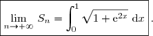
}{n}} }.)

+1=n\end{matrix}\right.)
}{n}} }=\dfrac 1 n\sum_{i=1}^{n}\sqrt{ 1+\text e^{\frac{2\,i}{n}} }=\dfrac 1 n\sum_{k=1}^{n}\sqrt{ 1+\text e^{\frac{2\,k}{n}} }.)
=\sqrt{1+\text e^{2x}}.)
 , on pose :
 }{n}\right)\quad\text{et}\quad S_{2,n}=\dfrac{b-a}{n}\sum_{k=1}^{n}f\left(a+\dfrac{k(b-a)}{n}\right))
 }) et
et  }) convergent et
convergent et \text{ d}x }\,.)
}{n}\right)=f\left(0+\dfrac{k(1-0)}{n}\right)=f\left(\dfrac{k}{n}\right)=\sqrt{1+\text e^{\frac{2k}{n}}} })
}{n}\right)=\dfrac{1-0}{n}\sum_{k=0}^{n-1}\sqrt{1+\text e^{\frac{2k}{n}}}\quad\Longrightarrow\quad \boxed{s_{1,n}=\dfrac{1}{n}\sum_{k=0}^{n-1}\sqrt{1+\text e^{\frac{2k}{n}}}}\\ \\ \text{et}\quad\displaystyle S_{2,n}=\dfrac{b-a}{n}\sum_{k=1}^{n}f\left(a+\dfrac{k(b-a)}{n}\right)=\dfrac{1-0}{n}\sum_{k=1}^{n}\sqrt{1+\text e^{\frac{2k}{n}}}\quad\Longrightarrow\quad \boxed{S_{2,n}=\dfrac{1}{n}\sum_{k=1}^{n}\sqrt{1+\text e^{\frac{2k}{n}}}})
\text{ d}x\le \lim\limits_{n\to+\infty}\,S_n\le\displaystyle\int_{0}^{1}f(x)\text{ d}x \\ \\ \phantom{W}\quad\Longrightarrow\quad \displaystyle\int_{0}^{1}\sqrt{1+\text e^{2x}}\text{ d}x\le \lim\limits_{n\to+\infty}\,S_n\le\displaystyle\int_{0}^{1}\sqrt{1+\text e^{2x}}\text{ d}x)
\text i\,. })
 et
et 
 Écrivons d'abord
  sous forme trigonométrique, soit sous la forme
 . })
^2}=\sqrt 2.)
![z_1=1-\text i=\sqrt 2\left(\dfrac{1}{\sqrt 2}-\dfrac{1}{\sqrt 2}\text i\right)\quad\Longrightarrow\quad z_1=\sqrt 2\left(\dfrac{\sqrt 2}{2}-\dfrac{\sqrt 2}{2}\text i\right) \\\\\text{D'où }\;\left\lbrace\begin{matrix}\cos\theta_1=\dfrac{\sqrt 2}{2}\\\overset{ { \white{ . } } } { \sin\theta_1=-\dfrac{\sqrt 2}{2}}\end{matrix}\right.\quad\Longrightarrow\quad\theta_1=-\dfrac{\pi}{4}\,[2\pi]](https://latex.ilemaths.net/latex-0.tex?z_1=1-\text i=\sqrt 2\left(\dfrac{1}{\sqrt 2}-\dfrac{1}{\sqrt 2}\text i\right)\quad\Longrightarrow\quad z_1=\sqrt 2\left(\dfrac{\sqrt 2}{2}-\dfrac{\sqrt 2}{2}\text i\right) \\\\\text{D'où }\;\left\lbrace\begin{matrix}\cos\theta_1=\dfrac{\sqrt 2}{2}\\\overset{ { \white{ . } } } { \sin\theta_1=-\dfrac{\sqrt 2}{2}}\end{matrix}\right.\quad\Longrightarrow\quad\theta_1=-\dfrac{\pi}{4}\,[2\pi])
 est :
est : ![\overset{ { \white{ . } } } { z_1=\sqrt 2\left[\cos\left(-\dfrac{\pi}{4}\right)+\text i\sin\left(-\dfrac{\pi}{4}\right)\right] }](https://latex.ilemaths.net/latex-0.tex?\overset{ { \white{ . } } } { z_1=\sqrt 2\left[\cos\left(-\dfrac{\pi}{4}\right)+\text i\sin\left(-\dfrac{\pi}{4}\right)\right] })
 est :
est : 
 sous forme trigonométrique, soit sous la forme
 . })
^2}=\sqrt {1+3}=\sqrt 4 =2.)
![z_2=1+\sqrt 3\,\text i=2\left(\dfrac{1}{2}+\dfrac{\sqrt 3}{2}\text i\right) \\\\\text{D'où }\;\left\lbrace\begin{matrix}\cos\theta_2=\dfrac{1}{2}\\\overset{ { \white{ . } } } { \sin\theta_2=\dfrac{\sqrt 3}{2}}\end{matrix}\right.\quad\Longrightarrow\quad\theta_2=\dfrac{\pi}{3}\,[2\pi]](https://latex.ilemaths.net/latex-0.tex?z_2=1+\sqrt 3\,\text i=2\left(\dfrac{1}{2}+\dfrac{\sqrt 3}{2}\text i\right) \\\\\text{D'où }\;\left\lbrace\begin{matrix}\cos\theta_2=\dfrac{1}{2}\\\overset{ { \white{ . } } } { \sin\theta_2=\dfrac{\sqrt 3}{2}}\end{matrix}\right.\quad\Longrightarrow\quad\theta_2=\dfrac{\pi}{3}\,[2\pi])
 est :
est : ![\overset{ { \white{ . } } } { z_2=2\left[\cos\left(\dfrac{\pi}{3}\right)+\text i\sin\left(\dfrac{\pi}{3}\right)\right] }](https://latex.ilemaths.net/latex-0.tex?\overset{ { \white{ . } } } { z_2=2\left[\cos\left(\dfrac{\pi}{3}\right)+\text i\sin\left(\dfrac{\pi}{3}\right)\right] })
 est :
est : 
(1+\sqrt 3\,\text i)}{2\sqrt 2}=\text e^{\text i\frac{\pi}{12}}.)
(1+\sqrt 3\,\text i)}{2\sqrt 2}=\dfrac{\sqrt 2\,\text e^{-\text i\frac{\pi}{4}}\times2\,\text e^{\text i\frac{\pi}{3}}}{2\sqrt 2} \\ \overset{ { \white{ P } } } { \phantom{WWWWWWw}= \text e^{-i\frac{\pi}{4}}\times\text e^{\text i\frac{\pi}{3}}} \\ \overset{ { \white{ P } } } { \phantom{WWWWWWw}= \text e^{\text i(\frac{\pi}{3}-\frac{\pi}{4})}} \\ \overset{ { \white{ P } } } { \phantom{WWWWWWw}= \text e^{\text i(\frac{4\pi}{12}-\frac{3\pi}{12})}})
(1+\sqrt 3\,\text i)}{2\sqrt 2}=\text e^{\text i\frac{\pi}{12}} })
(1+\sqrt 3\,\text i)}{2\sqrt 2}=\text e^{\text i\frac{\pi}{12}} \quad\Longleftrightarrow\quad\dfrac{1+\sqrt 3\,\text i-\text i+\sqrt 3}{2\sqrt 2}=\text e^{\text i\frac{\pi}{12}} \\ \overset{ { \white{ . } } } { \phantom{WWWWWWWWwW} \quad\Longleftrightarrow\quad\dfrac{\sqrt 3+1+(\sqrt 3 - 1)\,\text i}{2\sqrt 2}=\text e^{\text i\frac{\pi}{12}} } \\ \overset{ { \white{ . } } } { \phantom{WWWWWWWWwW} \quad\Longleftrightarrow\quad\dfrac{\sqrt 3+1}{2\sqrt 2}+\text i\dfrac{\sqrt 3-1}{2\sqrt 2}=\cos\left(\dfrac{\pi}{12}\right)+\text i \sin\left(\dfrac{\pi}{12}\right)})
=\dfrac{\sqrt 3+1}{2\sqrt 2}\\\overset{ { \white{ . } } } { \sin\left(\dfrac{\pi}{12}\right)=\dfrac{\sqrt 3-1}{2\sqrt 2}}\end{matrix}\right.)
=\dfrac{\sin\left(\dfrac{\pi}{12}\right)}{\cos\left(\dfrac{\pi}{12}\right)}=\dfrac{\dfrac{\sqrt 3-1}{2\sqrt 2}}{\dfrac{\sqrt 3+1}{2\sqrt 2}}=\dfrac{\sqrt 3-1}{\sqrt 3+1}=\dfrac{(\sqrt 3-1)^2}{(\sqrt 3+1)(\sqrt 3-1)} \\\\\phantom{WWWk}=\dfrac{3-2\sqrt 3+1}{(\sqrt 3)^2-1^2}=\dfrac{4-2\sqrt 3}{3-1}=\dfrac{2(2-\sqrt 3)}{2}=2-\sqrt 3 \\ \\ \\ \Longrightarrow\quad\boxed{\tan\left(\dfrac{\pi}{12}\right)=2-\sqrt 3 })
\text i=1+\text i \tan\left(\dfrac{\pi}{12}\right) \\ \overset{ { \white{ . } } } { \phantom{u}=1+\dfrac{\text i \sin\left(\dfrac{\pi}{12}\right)}{\cos\left(\dfrac{\pi}{12}\right)}=\dfrac{\cos\left(\dfrac{\pi}{12}\right)+\text i \sin\left(\dfrac{\pi}{12}\right)}{\cos\left(\dfrac{\pi}{12}\right)} })
} =\dfrac{1}{\cos\left(\dfrac{\pi}{12}\right)} \,\text e^{\text i\frac{\pi}{12}}=\dfrac{1}{\dfrac{\sqrt 3+1}{2\sqrt 2}} \,\text e^{\text i\frac{\pi}{12}}=\dfrac{2\sqrt 2}{\sqrt 3+1} \,\text e^{\text i\frac{\pi}{12}}} \\ \overset{ { \white{ . } } } { \phantom{u}=\dfrac{2\sqrt 2(\sqrt 3 -1)}{(\sqrt 3+1)(\sqrt 3 -1)} \,\text e^{\text i\frac{\pi}{12}}})
}{3-1} \,\text e^{\text i\frac{\pi}{12}}=\dfrac{2(\sqrt 6 -\sqrt 2)}{2} \,\text e^{\text i\frac{\pi}{12}}=(\sqrt 6 -\sqrt 2)\,\text e^{\text i\frac{\pi}{12}}} \\ \\ \\ \Longrightarrow\quad\boxed{u=(\sqrt 6 -\sqrt 2)\,\text e^{\text i\frac{\pi}{12}}})
_{n\in\N} }) et
et _{n\in\N} }) définies par :
définies par : 
\;\left\lbrace\begin{matrix}x_{n+1}=x_n-(2-\sqrt 3)y_n\\y_{n+1}=(2-\sqrt 3)x_n+y_n\end{matrix}\right.)

 , alors
y_n+\text i\left(\overset{}{(2-\sqrt 3)x_n+y_n}\right) \\ \overset{ { \white{ . } } } { \phantom{x_{n+1}+\text i y_{n+1}}=x_n-(2-\sqrt 3)y_n+\text i(2-\sqrt 3)x_n+\text iy_n} \\ \overset{ { \white{ . } } } { \phantom{x_{n+1}+\text i y_{n+1}}=x_n+\text iy_n+\text i(2-\sqrt 3)x_n-(2-\sqrt 3)y_n} \\ \overset{ { \white{ . } } } { \phantom{x_{n+1}+\text i y_{n+1}}=x_n+\text iy_n+\text i(2-\sqrt 3)\left(x_n-\dfrac{1}{\text i}\,y_n\right)})
(x_n+\text i\,y_n)} \\ \overset{ { \white{ . } } } { \phantom{x_{n+1}+\text i y_{n+1}}=(x_n+\text iy_n)\left(\overset{}{1+\text i(2-\sqrt 3)}\right)} \\ \overset{ { \white{ . } } } { \phantom{x_{n+1}+\text i y_{n+1}}=u^n\times u} \\ \overset{ { \phantom{ . } } } { \phantom{x_{n+1}+\text i y_{n+1}}=u^{n+1}} \\\\\Longrightarrow\quad\boxed{ x_{n+1}+\text i y_{n+1}=u^{n+1}})

![x_n+\text i y_n=u^n \\ \overset{ { \white{ . } } } { \phantom{WWWx}=\left[(\sqrt 6 -\sqrt 2)\,\text e^{\text i\frac{\pi}{12}}\right]^n \quad(\text{voir question 1. d})} \\ \overset{ { \white{ . } } } { \phantom{WWWx}=(\sqrt 6 -\sqrt 2)^n\,\text e^{\text i\frac{n\pi}{12}}} \\ \overset{ { \white{ . } } } { \phantom{WWWx}=(\sqrt 6 -\sqrt 2)^n\,\left(\cos\left(\dfrac{n\pi}{12}\right)+\text i \sin\left(\dfrac{n\pi}{12}\right)\right)}](https://latex.ilemaths.net/latex-0.tex?x_n+\text i y_n=u^n \\ \overset{ { \white{ . } } } { \phantom{WWWx}=\left[(\sqrt 6 -\sqrt 2)\,\text e^{\text i\frac{\pi}{12}}\right]^n \quad(\text{voir question 1. d})} \\ \overset{ { \white{ . } } } { \phantom{WWWx}=(\sqrt 6 -\sqrt 2)^n\,\text e^{\text i\frac{n\pi}{12}}} \\ \overset{ { \white{ . } } } { \phantom{WWWx}=(\sqrt 6 -\sqrt 2)^n\,\left(\cos\left(\dfrac{n\pi}{12}\right)+\text i \sin\left(\dfrac{n\pi}{12}\right)\right)})
^n\,\left(\cos\left(\dfrac{n\pi}{12}\right)+\text i \sin\left(\dfrac{n\pi}{12}\right)\right)} \\\phantom{WWWWWWWWWWWW}\quad\quad\text{car }\sqrt 6 -\sqrt 2=\dfrac{1}{\cos\dfrac{\pi}{12}}\quad\text{(voir question 1. d)} \\ \overset{ { \white{ . } } } {\Longrightarrow\boxed{x_n+\text i y_n=\dfrac{\cos\left(\dfrac{n\pi}{12}\right)}{\left(\cos\dfrac{\pi}{12}\right)^n}+\text i \dfrac{\sin\left(\dfrac{n\pi}{12}\right)}{\left(\cos\dfrac{\pi}{12}\right)^n}} })
}{\left(\cos\dfrac{\pi}{12}\right)^n}\\\\y_n= \dfrac{\sin\left(\dfrac{n\pi}{12}\right)}{\left(\cos\dfrac{\pi}{12}\right)^n}\end{matrix}\right.})
.)
 le point d'affixe
 et
et 
}{\left(\cos\dfrac{\pi}{12}\right)^n}=0)

=0 \\ \phantom{\text{Or }\;\dfrac{z_{A_n}-z_O}{z_{A_0}- z_O}\in\R}\quad\Longleftrightarrow\quad \exists\,k\in\Z\;:\; \dfrac{n\pi}{12}=k\pi \\ \phantom{\text{Or }\;\dfrac{z_{A_n}-z_O}{z_{A_0}- z_O}\in\R}\quad\Longleftrightarrow\quad \exists\,k\in\Z\;:\; \dfrac{n}{12}=k \\ \phantom{\text{Or }\;\dfrac{z_{A_n}-z_O}{z_{A_0}- z_O}\in\R}\quad\Longleftrightarrow\quad \exists\,k\in\Z\;:\; n=12k)
 et
et  sont distincts deux à deux.
 et
et 


}{-u^n}} \\ \overset{ { \white{ . } } } { \phantom{\text{Or }\;\dfrac{z_{A_{n+1}}-z_{A_n}}{z_0-z_{A_n}}}= \dfrac{u-1}{-1}} )

\text i\right)} )

\text i} )

 l'équation
 ![\overset{ { \white{ . } } } { (E):x^2\equiv 2\,[p]. }](https://latex.ilemaths.net/latex-0.tex?\overset{ { \white{ . } } } { (E):x^2\equiv 2\,[p]. })
![\overset{ { \white{ . } } } { 2^{p-1}\equiv 1\,[p]. }](https://latex.ilemaths.net/latex-0.tex?\overset{ { \white{ . } } } { 2^{p-1}\equiv 1\,[p]. })

 , alors
 ![\overset{ { \white{ . } } } { \boxed{2^{p-1}\equiv 1\,[p]}\,. }](https://latex.ilemaths.net/latex-0.tex?\overset{ { \white{ . } } } { \boxed{2^{p-1}\equiv 1\,[p]}\,. })
\left(2^{\frac{p-1}{2}}+1\right)=\left(2^{\frac{p-1}{2}}\right)^2-1^2\quad\Longrightarrow\quad \boxed{\left(2^{\frac{p-1}{2}}-1\right)\left(2^{\frac{p-1}{2}}+1\right)=2^{p-1}-1})

![2^{p-1}\equiv1\,[p]\quad\Longleftrightarrow\quad2^{p-1}-1\equiv0\,[p] \\ \overset{ { \white{ . } } } { \phantom{WWWwW} \quad\Longleftrightarrow\quad\left(2^{\frac{p-1}{2}}-1\right)\left(2^{\frac{p-1}{2}}+1\right)\equiv0\,[p]} \\ \overset{ { \white{ . } } } { \phantom{WWWwW} \quad\Longleftrightarrow\quad p\; | \left(2^{\frac{p-1}{2}}-1\right)\left(2^{\frac{p-1}{2}}+1\right)} \\ \overset{ { \white{ . } } } { \phantom{WWWwW} \quad\Longleftrightarrow\quad p\; |\, 2^{\frac{p-1}{2}}-1\quad\text{ou}\quad p\,|\,2^{\frac{p-1}{2}}+1}\quad\text{car }p\text{ est premier}](https://latex.ilemaths.net/latex-0.tex?2^{p-1}\equiv1\,[p]\quad\Longleftrightarrow\quad2^{p-1}-1\equiv0\,[p] \\ \overset{ { \white{ . } } } { \phantom{WWWwW} \quad\Longleftrightarrow\quad\left(2^{\frac{p-1}{2}}-1\right)\left(2^{\frac{p-1}{2}}+1\right)\equiv0\,[p]} \\ \overset{ { \white{ . } } } { \phantom{WWWwW} \quad\Longleftrightarrow\quad p\; | \left(2^{\frac{p-1}{2}}-1\right)\left(2^{\frac{p-1}{2}}+1\right)} \\ \overset{ { \white{ . } } } { \phantom{WWWwW} \quad\Longleftrightarrow\quad p\; |\, 2^{\frac{p-1}{2}}-1\quad\text{ou}\quad p\,|\,2^{\frac{p-1}{2}}+1}\quad\text{car }p\text{ est premier})
![\\ { \white{ . } } \overset{ { \white{ . } } } { \phantom{WWwwW} \quad\Longleftrightarrow\quad 2^{\frac{p-1}{2}}-1\equiv0\,[p]\quad\text{ou}\quad 2^{\frac{p-1}{2}}+1\equiv0\,[p]} \\ \overset{ { \white{ . } } } { \phantom{WWWwW} \quad\Longleftrightarrow\quad \boxed{ 2^{\frac{p-1}{2}}\equiv1\,[p]\quad\text{ou}\quad 2^{\frac{p-1}{2}}\equiv-1\,[p] }}](https://latex.ilemaths.net/latex-0.tex?\\ { \white{ . } } \overset{ { \white{ . } } } { \phantom{WWwwW} \quad\Longleftrightarrow\quad 2^{\frac{p-1}{2}}-1\equiv0\,[p]\quad\text{ou}\quad 2^{\frac{p-1}{2}}+1\equiv0\,[p]} \\ \overset{ { \white{ . } } } { \phantom{WWWwW} \quad\Longleftrightarrow\quad \boxed{ 2^{\frac{p-1}{2}}\equiv1\,[p]\quad\text{ou}\quad 2^{\frac{p-1}{2}}\equiv-1\,[p] }})
![x^2\equiv 2\,[p]](https://latex.ilemaths.net/latex-0.tex?x^2\equiv 2\,[p]) , soit que
, soit que ![x^2-2\equiv 0\,[p]](https://latex.ilemaths.net/latex-0.tex?x^2-2\equiv 0\,[p]) .
.
![\left\lbrace\begin{matrix}p\,|\,x^2\phantom{xxx}\\\overset{ { \white{ . } } } { p\,|\,x^2-2}\end{matrix}\right.\quad\Longrightarrow\quad p\,|\,[x^2-(x^2-2)] \\ \overset{ { \white{ . } } } { \phantom{WWiWW}\quad\Longrightarrow\quad p\,|\,(x^2-x^2+2)} \\ \overset{ { \white{ . } } } { \phantom{WWiWW}\quad\Longrightarrow\quad p\,|\,2}](https://latex.ilemaths.net/latex-0.tex?\left\lbrace\begin{matrix}p\,|\,x^2\phantom{xxx}\\\overset{ { \white{ . } } } { p\,|\,x^2-2}\end{matrix}\right.\quad\Longrightarrow\quad p\,|\,[x^2-(x^2-2)] \\ \overset{ { \white{ . } } } { \phantom{WWiWW}\quad\Longrightarrow\quad p\,|\,(x^2-x^2+2)} \\ \overset{ { \white{ . } } } { \phantom{WWiWW}\quad\Longrightarrow\quad p\,|\,2})
 .
.![2^{\frac{p-1}{2}}\equiv 1\,[p]\,.](https://latex.ilemaths.net/latex-0.tex?2^{\frac{p-1}{2}}\equiv 1\,[p]\,.)

![\overset{ { \white{ . } } } { \boxed{x^{p-1}\equiv 1\,[p]}\,. }](https://latex.ilemaths.net/latex-0.tex?\overset{ { \white{ . } } } { \boxed{x^{p-1}\equiv 1\,[p]}\,. })

![x^2\equiv 2\,[p]\quad\Longrightarrow\quad \left(x^2\right)^{\frac{p-1}{2}}\equiv 2^{\frac{p-1}{2}}\,[p] \\ \overset{ { \white{ . } } } { \phantom{x^2\equiv 2\,[p]}\quad\Longrightarrow\quad \boxed{x^{p-1}\equiv 2^{\frac{p-1}{2}}\,[p] } }](https://latex.ilemaths.net/latex-0.tex?x^2\equiv 2\,[p]\quad\Longrightarrow\quad \left(x^2\right)^{\frac{p-1}{2}}\equiv 2^{\frac{p-1}{2}}\,[p] \\ \overset{ { \white{ . } } } { \phantom{x^2\equiv 2\,[p]}\quad\Longrightarrow\quad \boxed{x^{p-1}\equiv 2^{\frac{p-1}{2}}\,[p] } }) .
.![\left\lbrace\begin{matrix}x^{p-1}\equiv 2^{\frac{p-1}{2}}\,[p]\\\overset{ { \white{ . } } } { x^{p-1}\equiv 1\,[p] }\end{matrix}\right.\quad\Longleftrightarrow\quad\left\lbrace\begin{matrix}2^{\frac{p-1}{2}}\equiv {\red{x^{p-1}}}\,[p]\\\overset{ { \white{ . } } } { {\red{x^{p-1}}}\equiv 1\,[p] }\end{matrix}\right.\quad\Longrightarrow\quad\boxed{2^{\frac{p-1}{2}}\equiv 1\,[p]}\,.](https://latex.ilemaths.net/latex-0.tex?\left\lbrace\begin{matrix}x^{p-1}\equiv 2^{\frac{p-1}{2}}\,[p]\\\overset{ { \white{ . } } } { x^{p-1}\equiv 1\,[p] }\end{matrix}\right.\quad\Longleftrightarrow\quad\left\lbrace\begin{matrix}2^{\frac{p-1}{2}}\equiv {\red{x^{p-1}}}\,[p]\\\overset{ { \white{ . } } } { {\red{x^{p-1}}}\equiv 1\,[p] }\end{matrix}\right.\quad\Longrightarrow\quad\boxed{2^{\frac{p-1}{2}}\equiv 1\,[p]}\,.)

\,!}\quad\Longleftrightarrow\quad C_p^k=\dfrac{p(p-1)\,!}{k(k-1)\,!(p-k)\,!} \\ \overset{ { \white{ . } } } { \phantom{WWWWWWWWWWWWWWWiW}\quad\Longleftrightarrow\quad k\,C_p^k=p\times\dfrac{(p-1)\,!}{(k-1)\,!(p-k)\,!} } \\ \overset{ { \white{ . } } } { \phantom{WWWWWWWWWWWWWWWiW}\quad\Longleftrightarrow\quad k\,C_p^k=p\, C_{p-1}^{k-1} } \\ \overset{ { \white{ . } } } { \phantom{WWWWWWWWWWWWWWWiW}\quad\Longrightarrow\quad p\,|\,k\,C_p^k })
\,.})

 et que p est premier avec k .
^p=2^{\frac p 2 }\cos\left(p\dfrac{\pi}{4}\right)+\text i\,2^{\frac p 2 }\sin\left(p\dfrac{\pi}{4}\right).})
 \\ \overset{ { \white{ . } } } { \phantom{1+\text i}=\sqrt 2\left(\dfrac{\sqrt 2 }{2}+\text i\,\dfrac{\sqrt 2 }{2}\right) } \\ \overset{ { \white{ . } } } { \phantom{1+\text i}=\sqrt 2\left(\cos\left(\dfrac{\pi }{4}\right)+\text i\,\sin\left(\dfrac{\pi }{4}\right)\right) })
![\\ \\ \Longrightarrow(1+\text i)^p=\left[\sqrt 2\left(\cos\left(\dfrac{\pi }{4}\right)+\text i\,\sin\left(\dfrac{\pi }{4}\right)\right)\right]^p \\ \overset{ { \white{ . } } } { \phantom{WWWxW} =\left(\sqrt 2\right)^p\left(\cos\left(\dfrac{\pi }{4}\right)+\text i\,\sin\left(\dfrac{\pi }{4}\right)\right) ^p } \\ \overset{ { \white{ . } } } { \phantom{WWWxW} =\left(2^{\frac 1 2}\right)^p\left(\cos\left(\dfrac{\pi }{4}\right)+\text i\,\sin\left(\dfrac{\pi }{4}\right)\right) ^p } \\ \overset{ { \white{ . } } } { \phantom{WWWxW} =2^{\frac p 2}\left(\cos\left(p\,\dfrac{\pi }{4}\right)+\text i\,\sin\left(p\,\dfrac{\pi }{4}\right)\right) }\quad\quad(\text{en utilisant la formule de Moivre)}](https://latex.ilemaths.net/latex-0.tex?\\ \\ \Longrightarrow(1+\text i)^p=\left[\sqrt 2\left(\cos\left(\dfrac{\pi }{4}\right)+\text i\,\sin\left(\dfrac{\pi }{4}\right)\right)\right]^p \\ \overset{ { \white{ . } } } { \phantom{WWWxW} =\left(\sqrt 2\right)^p\left(\cos\left(\dfrac{\pi }{4}\right)+\text i\,\sin\left(\dfrac{\pi }{4}\right)\right) ^p } \\ \overset{ { \white{ . } } } { \phantom{WWWxW} =\left(2^{\frac 1 2}\right)^p\left(\cos\left(\dfrac{\pi }{4}\right)+\text i\,\sin\left(\dfrac{\pi }{4}\right)\right) ^p } \\ \overset{ { \white{ . } } } { \phantom{WWWxW} =2^{\frac p 2}\left(\cos\left(p\,\dfrac{\pi }{4}\right)+\text i\,\sin\left(p\,\dfrac{\pi }{4}\right)\right) }\quad\quad(\text{en utilisant la formule de Moivre)})
^p=2^{\frac p 2 }\cos\left(p\dfrac{\pi}{4}\right)+\text i\,2^{\frac p 2 }\sin\left(p\dfrac{\pi}{4}\right).} })
^p =\displaystyle\sum_{k=0}^{k=\frac{p-1}{2}} (-1)^kC_p^{2k}+\text i\,\sum_{k=0}^{k=\frac{p-1}{2}} (-1)^kC_p^{2k+1}\,. )
\in\Z }) et que
et que ![\overset{ { \white{ . } } } { 2^{\frac p 2 }\cos\left(p\dfrac{\pi}{4}\right)\equiv 1\,[p].}](https://latex.ilemaths.net/latex-0.tex?\overset{ { \white{ . } } } { 2^{\frac p 2 }\cos\left(p\dfrac{\pi}{4}\right)\equiv 1\,[p].})
^p=2^{\frac p 2 }\cos\left(p\dfrac{\pi}{4}\right)+\text i\,2^{\frac p 2 }\sin\left(p\dfrac{\pi}{4}\right) \quad\text{(voir 4.a)}}\phantom{}\\\overset{ { \white{ . } } } { (1+\text i)^p =\displaystyle\sum_{k=0}^{k=\frac{p-1}{2}} (-1)^kC_p^{2k}+\text i\,\sum_{k=0}^{k=\frac{p-1}{2}} (-1)^kC_p^{2k+1} }\end{matrix}\right.)
=\displaystyle\sum_{k=0}^{k=\frac{p-1}{2}} (-1)^kC_p^{2k}\,.)
^k\in\Z\\\overset{ { \white{ . } } } { C_p^{2k}\in\N }\end{matrix}\right.\quad\Longrightarrow\quad(-1)^kC_p^{2k}\in\Z \\\\\text{D'où }\;\displaystyle\sum_{k=0}^{k=\frac{p-1}{2}} (-1)^kC_p^{2k}\in\Z.)
\in\Z} })

 , soit
 ![\overset{ { \white{ . } } } { C_p^{2k}\equiv 0\,[p] }](https://latex.ilemaths.net/latex-0.tex?\overset{ { \white{ . } } } { C_p^{2k}\equiv 0\,[p] })
![\forall\,k\in\lbrace1,2,\cdots,\dfrac{p-1}{2}\rbrace,\;C_p^{2k}\equiv 0\,[p]\quad\Longrightarrow\quad(-1)^kC_p^{2k}\equiv 0\,[p] \\ \overset{ { \white{ . } } } { \phantom{WWWWWWWWWWWWWW}\quad\Longrightarrow\quad\displaystyle\sum_{k=1}^{k=\frac{p-1}{2}} (-1)^kC_p^{2k}\equiv 0\,[p] } \\ \overset{ { \white{ . } } } { \phantom{WWWWWWWWWWWWWW}\quad\Longrightarrow\quad(-1)^0C_p^{0}+\displaystyle\sum_{k=1}^{k=\frac{p-1}{2}} (-1)^kC_p^{2k}\equiv (-1)^0C_p^{0}\,[p] } \\ \overset{ { \white{ . } } } { \phantom{WWWWWWWWWWWWWW}\quad\Longrightarrow\quad\displaystyle\sum_{k={\red{0}}}^{k=\frac{p-1}{2}} (-1)^kC_p^{2k}\equiv 1\,[p] }](https://latex.ilemaths.net/latex-0.tex?\forall\,k\in\lbrace1,2,\cdots,\dfrac{p-1}{2}\rbrace,\;C_p^{2k}\equiv 0\,[p]\quad\Longrightarrow\quad(-1)^kC_p^{2k}\equiv 0\,[p] \\ \overset{ { \white{ . } } } { \phantom{WWWWWWWWWWWWWW}\quad\Longrightarrow\quad\displaystyle\sum_{k=1}^{k=\frac{p-1}{2}} (-1)^kC_p^{2k}\equiv 0\,[p] } \\ \overset{ { \white{ . } } } { \phantom{WWWWWWWWWWWWWW}\quad\Longrightarrow\quad(-1)^0C_p^{0}+\displaystyle\sum_{k=1}^{k=\frac{p-1}{2}} (-1)^kC_p^{2k}\equiv (-1)^0C_p^{0}\,[p] } \\ \overset{ { \white{ . } } } { \phantom{WWWWWWWWWWWWWW}\quad\Longrightarrow\quad\displaystyle\sum_{k={\red{0}}}^{k=\frac{p-1}{2}} (-1)^kC_p^{2k}\equiv 1\,[p] })
=\displaystyle\sum_{k=0}^{k=\frac{p-1}{2}} (-1)^kC_p^{2k}\,,) nous en déduisons que
nous en déduisons que ![\overset{ { \white{ . } } } { \boxed{2^{\frac p 2 }\cos\left(p\dfrac{\pi}{4}\right)\equiv 1\,[p].}}](https://latex.ilemaths.net/latex-0.tex?\overset{ { \white{ . } } } { \boxed{2^{\frac p 2 }\cos\left(p\dfrac{\pi}{4}\right)\equiv 1\,[p].}})
![\overset{ { \white{ . } } } { p\equiv 5\,[8] }](https://latex.ilemaths.net/latex-0.tex?\overset{ { \white{ . } } } { p\equiv 5\,[8] }) , alors l'équation
, alors l'équation  }) n'a pas de solution dans
n'a pas de solution dans 
![p\equiv5\,[8]\quad\Longleftrightarrow\quad\exists \,k\in\Z : p=5+8k.](https://latex.ilemaths.net/latex-0.tex?p\equiv5\,[8]\quad\Longleftrightarrow\quad\exists \,k\in\Z : p=5+8k.)
\,. })
![\overset{ { \white{ . } } } { 2^{\frac p 2 }\cos\left(p\dfrac{\pi}{4}\right)\equiv 1\,[p].}](https://latex.ilemaths.net/latex-0.tex?\overset{ { \white{ . } } } { 2^{\frac p 2 }\cos\left(p\dfrac{\pi}{4}\right)\equiv 1\,[p].})
![2^{\frac p 2 }\cos\left(p\dfrac{\pi}{4}\right)\equiv 1\,[p]\quad\Longleftrightarrow\quad 2^{\frac p 2 }\cos\left((5+8k)\dfrac{\pi}{4}\right)\equiv 1\,[p] \\ \overset{ { \white{ . } } } { \phantom{WWWWWWWX}\quad\Longleftrightarrow\quad 2^{\frac p 2 }\cos\left(\dfrac{5\pi}{4}+2\pi\right)\equiv 1\,[p]} \\ \overset{ { \white{ . } } } { \phantom{WWWWWWWX}\quad\Longleftrightarrow\quad 2^{\frac p 2 }\cos\left(\dfrac{5\pi}{4}\right)\equiv 1\,[p]} \\ \overset{ { \white{ . } } } { \phantom{WWWWWWWX}\quad\Longleftrightarrow\quad 2^{\frac p 2 }\times\left(-\dfrac{\sqrt 2}{2}\right)\equiv 1\,[p]}](https://latex.ilemaths.net/latex-0.tex?2^{\frac p 2 }\cos\left(p\dfrac{\pi}{4}\right)\equiv 1\,[p]\quad\Longleftrightarrow\quad 2^{\frac p 2 }\cos\left((5+8k)\dfrac{\pi}{4}\right)\equiv 1\,[p] \\ \overset{ { \white{ . } } } { \phantom{WWWWWWWX}\quad\Longleftrightarrow\quad 2^{\frac p 2 }\cos\left(\dfrac{5\pi}{4}+2\pi\right)\equiv 1\,[p]} \\ \overset{ { \white{ . } } } { \phantom{WWWWWWWX}\quad\Longleftrightarrow\quad 2^{\frac p 2 }\cos\left(\dfrac{5\pi}{4}\right)\equiv 1\,[p]} \\ \overset{ { \white{ . } } } { \phantom{WWWWWWWX}\quad\Longleftrightarrow\quad 2^{\frac p 2 }\times\left(-\dfrac{\sqrt 2}{2}\right)\equiv 1\,[p]})

![\\ \overset{ { \white{ . } } } { \phantom{WWWWWWWX}\quad\Longleftrightarrow\quad 2^{\frac p 2 }\times\left(-\dfrac{2^{\frac 1 2}}{2}\right)\equiv 1\,[p]} \\ \overset{ { \white{ . } } } { \phantom{WWWWWWWX}\quad\Longleftrightarrow\quad 2^{\frac p 2 }\times\left(-2^{-\frac 1 2}\right)\equiv 1\,[p]} \\ \overset{ { \white{ . } } } { \phantom{WWWWWWWX}\quad\Longleftrightarrow\quad -2^{\frac {p-1}{ 2} }\equiv 1\,[p]}](https://latex.ilemaths.net/latex-0.tex?\\ \overset{ { \white{ . } } } { \phantom{WWWWWWWX}\quad\Longleftrightarrow\quad 2^{\frac p 2 }\times\left(-\dfrac{2^{\frac 1 2}}{2}\right)\equiv 1\,[p]} \\ \overset{ { \white{ . } } } { \phantom{WWWWWWWX}\quad\Longleftrightarrow\quad 2^{\frac p 2 }\times\left(-2^{-\frac 1 2}\right)\equiv 1\,[p]} \\ \overset{ { \white{ . } } } { \phantom{WWWWWWWX}\quad\Longleftrightarrow\quad -2^{\frac {p-1}{ 2} }\equiv 1\,[p]})
![\\ \overset{ { \white{ . } } } { \phantom{WWWWWWWX}\quad\Longleftrightarrow\quad 2^{\frac {p-1}{ 2} }\equiv -1\,[p]}](https://latex.ilemaths.net/latex-0.tex?\\ \overset{ { \white{ . } } } { \phantom{WWWWWWWX}\quad\Longleftrightarrow\quad 2^{\frac {p-1}{ 2} }\equiv -1\,[p]})
![2^{\frac {p-1}{ 2} }\equiv 1\,[p]\,.](https://latex.ilemaths.net/latex-0.tex?2^{\frac {p-1}{ 2} }\equiv 1\,[p]\,.)
![\left\lbrace\begin{matrix}2^{\frac {p-1}{ 2} }\equiv -1\,[p]\\\overset{ { \white{ . } } } { 2^{\frac {p-1}{ 2} }\equiv 1\,[p]}\end{matrix}\right.\quad\Longrightarrow\quad1\equiv -1\,[p] \\ \phantom{WWWWiWW}\quad\Longrightarrow\quad2\equiv 0\,[p] \\\\ \phantom{WWWWiWW}\quad\Longrightarrow\quad p\,|\,2](https://latex.ilemaths.net/latex-0.tex?\left\lbrace\begin{matrix}2^{\frac {p-1}{ 2} }\equiv -1\,[p]\\\overset{ { \white{ . } } } { 2^{\frac {p-1}{ 2} }\equiv 1\,[p]}\end{matrix}\right.\quad\Longrightarrow\quad1\equiv -1\,[p] \\ \phantom{WWWWiWW}\quad\Longrightarrow\quad2\equiv 0\,[p] \\\\ \phantom{WWWWiWW}\quad\Longrightarrow\quad p\,|\,2)
,+,\times)}) est un anneau non commutatif de zéro la matrice
est un anneau non commutatif de zéro la matrice  et d'unité la matrice
  , et que
 ,+,.)}) est un espace vectoriel réel.
est un espace vectoriel réel.=\begin{pmatrix}x+y&y\\2y&x-y\end{pmatrix}\;/\;(x,y)\in\R^2\right\rbrace\,.})
 est un sous-groupe de
 ,+)\,.})
,+)}) est un groupe car
est un groupe car  est un sous-groupe de
 }) comprend l'élément neutre du groupe
comprend l'élément neutre du groupe 
=\begin{pmatrix}x+y&y\\2y&x-y\end{pmatrix}\in E\quad\text{avec } x=y=0. \\\overset{ { \white{ . } } } { \phantom{xxx} M(0,0)=\begin{pmatrix}0+0&0\\2\times0&0-0\end{pmatrix}\in E }\quad\Longrightarrow\quad M(0,0)=\begin{pmatrix}0&0\\0&0\end{pmatrix} \in E \\\phantom{WWWWWWWWWWWwW}\phantom{xxx}\quad\Longrightarrow\quad \boxed{O\in E})
\in E\text{ et }M'(x',y')\in E \\\overset{ { \white{ . } } } { \phantom{xxi} \text{Alors }\;M(x,y)-M'(x',y') }=\begin{pmatrix}x+y&y\\2y&x-y\end{pmatrix}-\begin{pmatrix}x'+y'&y'\\2y'&x'-y'\end{pmatrix} \\ \overset{ { \white{ . } } } { \phantom{WWWWWWWWWWWWi} =\begin{pmatrix}(x-x')+(y-y')&(y-y')\\2(y-y')&(x-x')-(y-y')\end{pmatrix} } \\ \overset{ { \white{ . } } } { \phantom{WWWWWWWWWWWWi} =M(x-x',y-y') \in E } \\\\\Longrightarrow\quad\boxed{\forall\,M(x,y)\in E,M'(x',y')\in E : M(x,y)-M'(x',y')\in E})
,+,.)\,.})
 } \\ \overset{ { \white{ . } } } { \bullet\quad O=M(0,0)\in E\quad\Longrightarrow\quad\boxed{ E\neq \phi} } \\ \overset{ { \white{ . } } } { \bullet\quad \forall\,M(x,y),M'(x',y')\in E\;\text{ et }\;\forall\alpha,\beta\in\R,\quad } \\ \overset{ { \white{ . } } } { \phantom{WWWW} \alpha M(x,y)+\beta M'(x',y')=\alpha\begin{pmatrix}x+y&y\\2y&x-y\end{pmatrix}+\beta\begin{pmatrix}x'+y'&y'\\2y'&x'-y'\end{pmatrix}} \\ \overset{ { \phantom{ . } } } { \phantom{WWWW\alpha M(x,y)+\beta M'(x',y')}=\begin{pmatrix}\alpha(x+y)&\alpha y\\2\alpha y&\alpha(x-y)\end{pmatrix}+\begin{pmatrix}\beta(x'+y')&\beta y'\\2\beta y'&\beta (x'-y')\end{pmatrix}})
+\beta M'(x',y')}=\begin{pmatrix}\alpha x+\alpha y&\alpha y\\2\alpha y&\alpha x-\alpha y\end{pmatrix}+\begin{pmatrix}\beta x'+\beta y'&\beta y'\\2\beta y'&\beta x'-\beta y'\end{pmatrix}} \\ \overset{ { \phantom{ . } } } { \phantom{WWWW\alpha M(x,y)+\beta M'(x',y')}=\begin{pmatrix}\alpha x+\alpha y+\beta x'+\beta y'&\alpha y+\beta y'\\2\alpha y+2\beta y'&\alpha x-\alpha y+\beta x'-\beta y'\end{pmatrix}} \\ \overset{ { \phantom{ . } } } { \phantom{WWWW\alpha M(x,y)+\beta M'(x',y')}=\begin{pmatrix}(\alpha x+\beta x')+(\alpha y+\beta y')&\alpha y+\beta y'\\2(\alpha y+\beta y')&(\alpha x+\beta x')-(\alpha y+\beta y')\end{pmatrix}} \\ \overset{ { \phantom{ . } } } { \phantom{WWWW\alpha M(x,y)+\beta M'(x',y')}=M(\alpha x+\beta x',\alpha y+\beta y')\in E} \\\\\Longrightarrow\quad\boxed{ \forall\,M(x,y),M'(x',y')\in E\;\text{ et }\;\forall\alpha,\beta\in\R,\quad \alpha M(x,y)+\beta M'(x',y')\in E})
 }}}\forall\;(x,x',y,y')\in\R^4: \\\\M(x,y)\times M'(x',y')=\begin{pmatrix}x+y&y\\2y&x-y\end{pmatrix}\times\begin{pmatrix}x'+y'&y'\\2y'&x'-y'\end{pmatrix} \\ \overset{ { \white{ . } } } { \phantom{WWWWWWWW}=\begin{pmatrix}(x+y)(x'+y')+2yy'&(x+y)y'+y(x'-y')\\2y(x'+y')+(x-y)2y'&2yy'+(x-y)(x'-y')\end{pmatrix} } \\ \overset{ { \white{ . } } } { \phantom{WWWWWWWW}=\begin{pmatrix}xx'+xy'+yx'+yy'+2yy'&xy'+yy'+yx'-yy'\\2yx'+2yy'+2xy'-2yy'&2yy'+xx'-xy'-yx'+yy'\end{pmatrix} } \\ \overset{ { \white{ . } } } { \phantom{WWWWWWWW}=\begin{pmatrix}xx'+xy'+yx'+3yy'&xy'+yx'\\2yx'+2xy'&xx'+3yy'-xy'-yx'\end{pmatrix} })
+(xy'+yx')&xy'+yx'\\2(xy'+yx')&(xx'+3yy')-(xy'+yx')\end{pmatrix} } \\ \overset{ { \white{ . } } } { \phantom{WWWWWWWW}=M(xx'+3yy',xy'+yx') } \\\\\Longrightarrow\quad\boxed{\forall\;(x,x',y,y')\in\R^4: M(x,y)\times M'(x',y')=M(xx'+3yy',xy'+yx') })
}) est un anneau commutatif et unitaire.
est un anneau commutatif et unitaire. Montrons que
 ,+,\times)\,.}) .
.
\,.)
 car
car \in E. })
\in E,M'(x',y')\in E : M(x,y)-M'(x',y')\in E) car
car ) est un groupe (voir question 1).
est un groupe (voir question 1).\in E,M'(x',y')\in E : M(x,y)\times M'(x',y')\in E) car cette propriété a été démontrée dans
car cette propriété a été démontrée dans  (voir question 3. a).
 est commutative dans
 \in E,M(x',y')\in E : \\ \\ M(x,y)\times M(x',y')= M(xx'+3yy',xy'+yx') \\ \overset{ { \white{ . } } } { \phantom{M(x,y)\times M'(x',y')}= M(x'x+3y'y,x'y+y'x) } \\ \overset{ { \white{ . } } } { \phantom{M(x,y)\times M'(x',y')}= M(x',y')\times M(x,y) } \\\\\Longrightarrow\boxed{\forall\,M(x,y)\in E,M(x',y')\in E :M(x,y)\times M(x',y')=M(x',y')\times M(x,y)} )
 nous en déduisons que
 \times M(-\sqrt 3, 1)=M\left(\overset{}{\sqrt 3\times(-\sqrt 3)+3\times1\times1,\sqrt 3\times1+1\times(-\sqrt 3)}\right) \\ \phantom{M(\sqrt 3,1)\times M(-\sqrt 3, 1)}=M\left(\overset{}{-3+3,\sqrt 3-\sqrt 3}\right) \\ \phantom{M(\sqrt 3,1)\times M(-\sqrt 3, 1)}=M\left(\overset{}{0,0}\right)=O \\\\\Longrightarrow\boxed{M(\sqrt 3,1)\times M(-\sqrt 3, 1)=O})
\times M(-\sqrt 3, 1)=O.)
\neq O) et
et \neq O)
) et
et ) sont des diviseurs de zéro.
sont des diviseurs de zéro.\in\Q^2\right\rbrace }) et
et =\begin{pmatrix}x+y&y\\2y&x-y\end{pmatrix}\,\left/\right\,(x,y)\in\Q^2\right\rbrace\;. })
\in\Q^2:x+y\sqrt 3=0\quad\Longleftrightarrow\quad(x=0\;\text{ et }\;y=0))
\in\Q^2:x+y\sqrt 3=0\quad\Longrightarrow\quad(x=0\;\text{ et }\;y=0))


 , ce qui est impossible puisque
  et
et 


\in\Q^2:x+y\sqrt 3=0\quad\Longrightarrow\quad(x=0\;\text{ et }\;y=0)\,.)
\in\Q^2:(x=0\;\text{ et }\;y=0)\quad\Longrightarrow\quad x+y\sqrt 3=0)
 C'est évident car
 \quad\Longrightarrow\quad x+y\sqrt 3=0+0\times\sqrt 3=0.)
\in\Q^2:x+y\sqrt 3=0\quad\Longleftrightarrow\quad(x=0\;\text{ et }\;y=0)})
 est un sous-groupe de
  })

 et que
 \times(x'+y'\sqrt 3)^{-1}\in F-\lbrace0\rbrace.})
\in\Q^2\\1\neq0\phantom{WWWWWWWWWWW}\end{matrix}\right.})
\times(x'+y'\sqrt 3)^{-1}=\dfrac{x+y\sqrt 3}{x'+y'\sqrt 3}} \\ \overset{ { \white{ . } } } {\phantom{XXXX(x+y\sqrt 3)\times(x'+y'\sqrt 3)^{-1}}=\dfrac{(x+y\sqrt 3)(x'-y'\sqrt 3)}{(x'+y'\sqrt 3)(x'-y'\sqrt 3)}} \\ \overset{ { \phantom{ . } } } {\phantom{XXXX(x+y\sqrt 3)\times(x'+y'\sqrt 3)^{-1}}=\dfrac{xx'-3yy'+yx'\sqrt 3-xy'\sqrt 3}{x'^2-3y'^2}} )

\times(x'+y'\sqrt 3)^{-1}}=\dfrac{xx'-3yy'}{x'^2-3y'^2}+\dfrac{yx'-xy'}{x'^2-3y'^2}\sqrt 3 \quad\quad \text{où }\left(\dfrac{xx'-3yy'}{x'^2-3y'^2},\dfrac{yx'-xy'}{x'^2-3y'^2}\right)\in\Q^2} \\\\\Longrightarrow\quad\boxed{(x+y\sqrt 3)\times(x'+y'\sqrt 3)^{-1}\in F})
^{-1}\neq0}\end{matrix}\right. \\ \\ \phantom{WWWWWWWWW}\quad\Longrightarrow\quad \boxed{(x+y\sqrt 3)\times(x'+y'\sqrt 3)^{-1}\neq0})
\times(x'+y'\sqrt 3)^{-1}\in F-\lbrace0\rbrace.}})
\,. })
 l'application définie de
  par :
par : \in\Q^2-\lbrace(0,0)\rbrace\,;\;\varphi(x+y\sqrt 3)=M(x,y)\,.})
=G-\lbrace O\rbrace.)
=\varphi\left(\overset{}{\lbrace x+y\sqrt 3\,/\,(x,y)\in\Q^2-\lbrace(0,0)\rbrace\rbrace}\right) \\ \phantom{\varphi(F-\lbrace 0\rbrace)}=\left\lbrace\overset{}{\varphi( x+y\sqrt 3)\,/\,(x,y)\in\Q^2-\lbrace(0,0)\rbrace}\right\rbrace \\ \phantom{\varphi(F-\lbrace 0\rbrace)}=\lbrace\overset{}{\varphi( x+y\sqrt 3)\,/\,(x,y)\in\Q^2\rbrace-\lbrace\varphi(0+0\sqrt 3)\rbrace} \\ \overset{ { \white{ . } } } { \phantom{\varphi(F-\lbrace 0\rbrace)}=\lbrace M(x,y)\,/\,(x,y)\in\Q^2\rbrace-\lbrace M(0,0)\rbrace} \\ \overset{ { \white{ . } } } { \phantom{\varphi(F-\lbrace 0\rbrace)}=G-\lbrace O\rbrace})
=G-\lbrace O\rbrace})
 }) vers
vers \,. })
\times(x'+y'\sqrt 3)}\right)=\varphi\left(\overset{}{(xx'+3yy'+(xy'+yx')\sqrt 3}\right)} \\ \overset{ { \white{ . } } } { \phantom{WWW \varphi\left(\overset{}{(x+y\sqrt 3)\times(x'+y'\sqrt 3)}\right)}=M(xx'+3yy',xy'+yx')} \\ \overset{ { \white{ . } } } { \phantom{WWW \varphi\left(\overset{}{(x+y\sqrt 3)\times(x'+y'\sqrt 3)}\right)}=M(x,y)\times M(x',y')\quad\quad(\text{voir question Partie I - 3. a)}})
\times(x'+y'\sqrt 3)}\right)}=\varphi(x+y\sqrt 3)\times \varphi(x'+y'\sqrt 3)} \\ \\ \Longrightarrow\quad\boxed{\begin{matrix}\forall\ x+y\sqrt 3,\,x'+y'\sqrt 3\in F-\lbrace 0\rbrace, \\\overset{ { \white{ . } } } { \varphi((x+y\sqrt 3)\times(x'+y'\sqrt 3))=\varphi(x+y\sqrt 3)\times \varphi(x'+y'\sqrt 3)}\end{matrix}\; })
 }) est un groupe commutatif.
est un groupe commutatif. }) est un groupe commutatif.
est un groupe commutatif.=G-\lbrace O\rbrace\,, }) nous déduisons que
nous déduisons que }) est un corps commutatif.
est un corps commutatif. Montrons que
 }) est un groupe commutatif.
est un groupe commutatif. Pour ce faire, montrons que
  est un sous-groupe commutatif de
 ,+)\,. })


 }) car
car 
\in G,M'(x',y')\in G : M(x,y)-M'(x',y')=M(x-x',y-y')\in G\,. })
 }) est un groupe commutatif.
est un groupe commutatif.. })
 Voir la correction
 forum de terminale