I. On considère la fonction polynôme définie dans par :
Nous devons exprimer sous forme de fonction rationnelle dont le dénominateur est un polynôme du premier degré.
L'expression de sera donnée sous cette forme.
L'expression représente la somme des premiers termes d'une suite géométrique de raison et de premier terme 1.
Cette somme est donnée par
Nous en déduisons que pour tout réel
soit
II. Un coureur s'entraîne sur un parcours comportant dix haies numérotées de 1 à 10.
Pour chaque entier tel que la probabilité de renverser la ième haie est
Le coureur poursuit sa course jusqu'à la 10ième haie, quel que soit le nombre de haies renversées.
Soit la variable aléatoire définie comme suit :
1. L'ensemble des valeurs prises par est
2. a) Pour chaque entier tel que la probabilité de renverser la ième haie est
Donc, la probabilité que le coureur renverse la première haie est égale à
2. b) Nous devons calculer la probabilité que le coureur renverse la deuxième haie pour la première fois, soit
Si le coureur renverse la deuxième haie pour la première fois, nous savons qu'il n'a pas renversé la première haie.
Dès lors,
Par conséquent, la probabilité que le coureur renverse la deuxième haie pour la première fois est
2. c) Pour chaque entier tel que la probabilité de renverser la ième haie est
Donc, la probabilité pour que le coureur renverse la deuxième haie est égale à
Remarque : Nous pouvons retrouver ce résultat en envisageant les deux cas possibles :
La première haie est renversée et la deuxième haie est également renversée. Dans ce cas, la probabilité que les deux haies soient renversées est égale à La première haie n'est pas renversée et la deuxième haie est renversée. Dans ce cas, la probabilité est égale à
Par conséquent, la probabilité pour que le coureur renverse la deuxième haie est égale à
3. a) Nous devons déterminer la loi de probabilité de
Pour chaque entier tel que si le coureur renverse la ième haie pour la première fois, il s'ensuit qu'il n'a pas renversé les haies précédentes.
Notons que si aucune des 10 haies n'a été renversée et
Nous obtenons ainsi le tableau suivant résumant la loi de probabilité de
3. b) Montrons que la somme des probabilités trouvées dans la loi de probabilité est égale à 1.
Appliquons le résultat de la question I. avec et nous obtenons :
Par conséquent, la somme des probabilités trouvées dans la loi de probabilité est égale à 1.
4. Le coureur reçoit la prime d'excellence s'il ne renverse aucune des 10 haies.
Nous devons calculer la probabilité que le coureur reçoive la prime d'excellence pour
Si le coureur ne renverse aucune des 10 haies, la valeur de est 11.
D'où la probabilité que le coureur reçoive la prime d'excellence est égale à environ 0,006, soit 0,6 %.
4 points
exercice 2
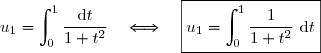
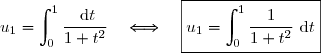
Soit la suite définie par
1. a) Montrons que la suite est croissante.
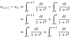
Pour tout entier naturel
Nous en déduisons que la suite est croissante.
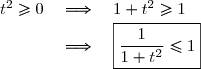
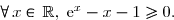
1. b) i. Montrons que pour tout réel
Pour tout réel
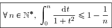
1. b) ii. Montrons que pour tout réel non nul
Pour tout réel non nul,
D'où pour tout réel non nul
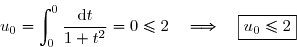
1. c) i. Montrons que
En utilisant le résultat de la question 1. b) i. , nous obtenons :
Par conséquent,
1. c) ii. Montrons que
En utilisant le résultat de la question 1. b) ii. , nous obtenons :
Par conséquent,
1. d) Montrons que la suite est majorée.
Pour tout
De plus,
Nous en déduisons que la suite est majorée par 2.
Nous avons montré que la suite est croissante et majorée.
Nous en déduisons que la suite est convergente.
2. Soit la fonction définie sur [0 ; +[
par : et
la fonction définie sur par
2. a) On pose
Nous devons démontrer que est dérivable sur
La fonction est la composée de la fonction et de la fonction
La fonction est dérivable sur et est à valeurs dans Montrons que la fonction est dérivable sur
La fonction est continue sur
Donc la fonction définie par : est l'unique primitive de qui s'annule en 0.
D'où la fonction est dérivable sur Nous en déduisons que la composée de et de est dérivable sur
Par conséquent, est dérivable sur
2. b) Nous devons déterminer
Nous en déduisons que où est une constante réelle.
Déterminons la valeur de la constante
Dès lors,
Par conséquent,
2. c) Nous savons que la fonction définie par est une bijection de dans et que
Par conséquent, la fonction est la fonction réciproque de la fonction et est définie sur par et est à valeurs dans l'intervalle
2. d) Nous devons déterminer
12 points
probleme
On considère la fonction définie sur ]1 ; +[ par :
On considère par la courbe représentative de dans un repère orthonormé
Partie A (6 points)
Dans cette partie, on étudie la fonction numérique définie sur ]0 ; +[ par :
1. Soit la fonction numérique définie sur par :
1. a) Montrons que admet un minimum en 0 qui est 0.
La fonction est dérivable sur (somme de fonctions dérivables sur ).
D'où le tableau de signes de sur et les variations de
Par conséquent, la fonction admet un minimum en 0 qui est 0.
1. b) D'après le tableau de variations de la fonction nous déduisons que
Dès lors,
Nous en déduisons que
2. a) Nous devons calculer pour tout
soit
2. b) Nous devons montrer que
Utilisons l'inégalité (1).
2. c) Nous devons en déduire le sens de variation de
Par conséquent, la fonction est strictement décroissante sur
3. a) Nous devons vérifier que
Pour tout ,
3. b) Soit la fonction numérique définie sur par Nous devons étudier les variations de
La fonction est dérivable sur comme somme de deux fonctions dérivables sur
D'où le tableau de signes de sur et les variations de
Par conséquent, la fonction est croissante sur .
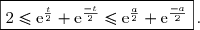
3. c) Soit
Nous devons démontrer que pour tout réel tel que nous avons :
La fonction est croissante sur et a fortiori sur
Donc pour tout réel tel que nous avons
soit
3. d) Remarque : l'énoncé comporte une coquille.
La relation correcte est :
Utilisons la question 3. c) et appliquons l'inégalité de la moyenne à la fonction sur
La fonction est continue sur
Nous obtenons alors :
D'où,
4. a) La relation (2) est valable pour tout réel
Par un changement d'écriture, nous obtenons alors : pour tout
Multiplions les trois membres de ces inégalités par
Nous obtenons ,
soit ,
soit
4. b) En utilisant l'inégalité (3), nous devons calculer
Calculons
Calculons , soit
Déterminons
En résumé,
Dès lors, par le théorème d'encadrement (théorème des gendarmes), nous obtenons :
Partie B (6 points)
1. a) Étudions la continuité de en 0.
D'une part,
D'autre part,
D'où
Par conséquent, nous obtenons :
Donc la fonction est continue en 0.
1. b) Étudions la dérivabilité de en 0.
Calculons
Posons
D'où
En outre,
Nous en déduisons que
Par conséquent, la fonction est dérivable à gauche en 0 et le nombre dérivé à gauche de en 0 est égal à
Étudions la dérivabilité à droite de en 0.
Par conséquent, la fonction est dérivable à droite en 0 et le nombre dérivé à droite de en 0 est égal à
Puisque les nombres dérivés à gauche et à droite de sont des nombres réels différents, nous en déduisons que la fonction n'est pas dérivable en 0.
Il s'ensuit graphiquement que la courbe admet un point anguleux de coordonnées (0 ; 1). De plus, au point de coordonnées (0 ; 1), la courbe admet une demi-tangente à gauche de coefficient directeur égal à 2 et une demi-tangente à droite de coefficient directeur égal à
2. Nous devons calculer et
Utilisons la relation (3) de la partie A.
Nous savons que
Par le théorème d'encadrement (théorème des gendarmes), nous obtenons :
3. a)Calculons sur
Calculons sur
Remarquons que
Donc
Dans la question 2. a) - Partie A, nous avons montré que
Dès lors,
3. b)Nous devons déterminer le sens de variation de sur
Par conséquent, est strictement croissante sur
Nous devons déterminer le sens de variation de sur
Remarquons que
Dans la question 2. c) - Partie A, nous avons conclu que la fonction est strictement décroissante sur
Par conséquent, la fonction est strictement décroissante sur
3. c) Dressons le tableau de variations de
4) Traçons la courbe
5. Soit la partie du plan délimitée par la courbe sur [0 ; +[, l'axe des abscisses et les droites d'équations et
Donnons un encadrement de l'aire en cm2.
Utilisons l'inégalité (3).
Selon l'énoncé, la mesure de l'unité graphique est égale à 3 cm.
Dès lors, l'unité d'aire est égale à 9 cm2.
Par conséquent,
soit
Publié par malou/Panter
le
ceci n'est qu'un extrait
Pour visualiser la totalité des cours vous devez vous inscrire / connecter (GRATUIT) Inscription Gratuitese connecter
Merci à Hiphigenie / Panter pour avoir contribué à l'élaboration de cette fiche
Désolé, votre version d'Internet Explorer est plus que périmée ! Merci de le mettre à jour ou de télécharger Firefox ou Google Chrome pour utiliser le site. Votre ordinateur vous remerciera !
 définie dans
  par :
par : =1+x+x^2+\cdots+x^{n-1}+x^n.} )
 } ) sera donnée sous cette forme.
sera donnée sous cette forme.=1+x+x^2+\cdots+x^{n-1}+x^n} ) représente la somme des
représente la somme des  premiers termes d'une suite géométrique de raison
  et de premier terme 1.
=\text{premier terme}\times\dfrac{1-\text{raison}^{\text{nombre de termes}}}{1-\text{raison}}.} )
=1\times\dfrac{1-x^{n+1}}{1-x})
=\dfrac{x^{n+1}-1}{x-1}}\,.)
 tel que
  la probabilité de renverser la
 . } )
 la variable aléatoire définie comme suit :


.} )
=(1-a)\times a.} )
=a(1-a)}\,.} )
 La première haie est renversée et la deuxième haie est également renversée.
 Dans ce cas, la probabilité que les deux haies soient renversées est égale à
\times a=a-a^2. } )
=\boxed{a}\,.} )

 si le coureur renverse la
  } ) haies précédentes.
haies précédentes. aucune des 10 haies n'a été renversée et
 =(1-a)^{10}. } )
&a&a(1-a)&a(1-a)^2&a(1-a)^3&\cdots&a(1-a)^7&a(1-a)^8&a(1-a)^9&(1-a)^{10}\\&&&&&&&&&\\ \hline \end{array})
 des probabilités trouvées dans la loi de probabilité est égale à 1.
+a(1-a)^2+a(1-a)^3+\cdots+a(1-a)^9+(1-a)^{10} \\\overset{ { \white{ . } } } { \phantom{S}=a\bigg(1+(1-a)+(1-a)^2+(1-a)^3+\cdots+(1-a)^9\bigg)+(1-a)^{10}})
 et
et  nous obtenons :
 ^{10}-1}{(1-a)-1}+(1-a)^{10} \\\overset{ { \white{ . } } } { \phantom{S}=a\times \dfrac{(1-a)^{10}-1}{-a}+(1-a)^{10}} \\\overset{ { \white{ . } } } { \phantom{S}= \dfrac{(1-a)^{10}-1}{-1}+(1-a)^{10}} \\\overset{ { \white{ . } } } { \phantom{S}= 1-(1-a)^{10}+(1-a)^{10}})

 est 11.
=(1-a)^{10} \\\overset{ { \white{ . } } } {\phantom{P(X=11)}=\left(1-\dfrac 2 5\right)^{10}} \\\overset{ { \white{ . } } } {\phantom{P(X=11)}=\left(\dfrac 3 5\right)^{10}\approx0,006} \\\\\quad\Longrightarrow\boxed{P(X=11)\approx0,006})
_{n\in\N}}) définie par
définie par 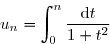
}) est croissante.
est croissante.
} \\\\\\\Longrightarrow\quad\boxed{\forall\,n\in\N,\; u_{n+1}-u_n\ge0})


 non nul,
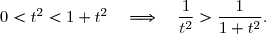

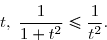
![\dfrac{1}{1+t^2}\le1\quad\Longrightarrow\quad \displaystyle\int_{0}^{1}\dfrac{1}{1+t^2}\text{ d}t\le\displaystyle\int_{0}^{1}1\text{ d}t \\\overset{ { \white{ . } } } {\phantom{\dfrac{1}{1+t^2}\le1}\quad\Longrightarrow\quad \displaystyle\int_{0}^{1}\dfrac{1}{1+t^2}\text{ d}t\le\left[\overset{ { \phantom{ . } } } { t}\right]_0^1} \\\overset{ { \white{ . } } } {\phantom{\dfrac{1}{1+t^2}\le1}\quad\Longrightarrow\quad \displaystyle\int_{0}^{1}\dfrac{1}{1+t^2}\text{ d}t\le 1-0} \\\overset{ { \phantom{ . } } } {\phantom{\dfrac{1}{1+t^2}\le1}\quad\Longrightarrow\quad \displaystyle\int_{0}^{1}\dfrac{1}{1+t^2}\text{ d}t\le 1}](https://latex.ilemaths.net/latex-0.tex?\dfrac{1}{1+t^2}\le1\quad\Longrightarrow\quad \displaystyle\int_{0}^{1}\dfrac{1}{1+t^2}\text{ d}t\le\displaystyle\int_{0}^{1}1\text{ d}t \\\overset{ { \white{ . } } } {\phantom{\dfrac{1}{1+t^2}\le1}\quad\Longrightarrow\quad \displaystyle\int_{0}^{1}\dfrac{1}{1+t^2}\text{ d}t\le\left[\overset{ { \phantom{ . } } } { t}\right]_0^1} \\\overset{ { \white{ . } } } {\phantom{\dfrac{1}{1+t^2}\le1}\quad\Longrightarrow\quad \displaystyle\int_{0}^{1}\dfrac{1}{1+t^2}\text{ d}t\le 1-0} \\\overset{ { \phantom{ . } } } {\phantom{\dfrac{1}{1+t^2}\le1}\quad\Longrightarrow\quad \displaystyle\int_{0}^{1}\dfrac{1}{1+t^2}\text{ d}t\le 1})

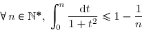
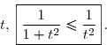
![\dfrac{1}{1+t^2}\le\dfrac{1}{t^2}\quad\Longrightarrow\quad \displaystyle\int_{1}^{n}\dfrac{1}{1+t^2}\text{ d}t\le\displaystyle\int_{1}^{n}\dfrac{1}{t^2}\text{ d}t \\\overset{ { \white{ . } } } {\phantom{\dfrac{1}{1+t^2}\le\dfrac{1}{t^2}}\quad\Longrightarrow\quad \displaystyle\int_{1}^{n}\dfrac{1}{1+t^2}\text{ d}t\le\left[\overset{ { \phantom{ . } } } {- \dfrac{1}{t}}\right]_{1}^{n}} \\\overset{ { \white{ . } } } {\phantom{\dfrac{1}{1+t^2}\le\dfrac{1}{t^2}}\quad\Longrightarrow\quad \displaystyle\int_{1}^{n}\dfrac{1}{1+t^2}\text{ d}t\le -\dfrac 1 n + 1} \\\overset{ { \phantom{ . } } } {\phantom{\dfrac{1}{1+t^2}\le\dfrac{1}{t^2}}\quad\Longrightarrow\quad \displaystyle\int_{1}^{n}\dfrac{1}{1+t^2}\text{ d}t\le 1-\dfrac 1 n}](https://latex.ilemaths.net/latex-0.tex?\dfrac{1}{1+t^2}\le\dfrac{1}{t^2}\quad\Longrightarrow\quad \displaystyle\int_{1}^{n}\dfrac{1}{1+t^2}\text{ d}t\le\displaystyle\int_{1}^{n}\dfrac{1}{t^2}\text{ d}t \\\overset{ { \white{ . } } } {\phantom{\dfrac{1}{1+t^2}\le\dfrac{1}{t^2}}\quad\Longrightarrow\quad \displaystyle\int_{1}^{n}\dfrac{1}{1+t^2}\text{ d}t\le\left[\overset{ { \phantom{ . } } } {- \dfrac{1}{t}}\right]_{1}^{n}} \\\overset{ { \white{ . } } } {\phantom{\dfrac{1}{1+t^2}\le\dfrac{1}{t^2}}\quad\Longrightarrow\quad \displaystyle\int_{1}^{n}\dfrac{1}{1+t^2}\text{ d}t\le -\dfrac 1 n + 1} \\\overset{ { \phantom{ . } } } {\phantom{\dfrac{1}{1+t^2}\le\dfrac{1}{t^2}}\quad\Longrightarrow\quad \displaystyle\int_{1}^{n}\dfrac{1}{1+t^2}\text{ d}t\le 1-\dfrac 1 n})


\quad\quad(\text{voir les questions 1.c) i. et ii.)} })
} \\\\\Longrightarrow\quad\boxed{\forall\,n\in\N^*,\;u_n\le2})
 définie sur [0 ; +
 [
par :
[
par : =\displaystyle\int_{0}^{x}\dfrac{\text{ d}t}{1+t^2} }) et
et
 la fonction définie sur
  par
par =\tan x.} )
=F(f(x)). } )
 Nous devons démontrer que
  est dérivable sur
 et de la fonction
 La fonction
 est dérivable sur
  est continue sur
  définie par :
  qui s'annule en 0.
 est dérivable sur
 .})
=\bigg((F\circ f)(x)\bigg)' \\\overset{ { \white{ . } } } {\phantom{G'(x)}=F'(f(x))\times f'(x) } \\\overset{ { \white{ . } } } {\phantom{G'(x)}=k(f(x))\times f'(x)\quad (\text{voir question }2. a)})
=\dfrac{1}{1+x^2}\quad\Longrightarrow\quad k(f(x))=\dfrac{1}{1+(f(x))^2} \\\overset{ { \white{ . } } } {\phantom{\text{Or }\;k(t)=\dfrac{1}{1+t^2}}\quad\Longrightarrow\quad k(f(x))=\dfrac{1}{1+\tan^2x}} \\\\\phantom{\text{Or }\;}f(x)=\tan x\quad\Longrightarrow\quad f'(x)=1+\tan^2x \\\\\text{D'où }\;G\,'(x)=\dfrac{1}{1+\tan^2x}\times (1+\tan^2x)\quad\Longrightarrow\quad\boxed{G\,'(x)=1})
=x+c}) où
où  est une constante réelle.
=F(f(x)) \quad\Longrightarrow\quad \boxed{G(0)=F(f(0))} } \\\\\text{Or }\;\left\lbrace\begin{matrix}f(0)=\tan 0\phantom{WWWWWWW}\quad\Longrightarrow\quad f(0)=0\\F(f(0))=F(0)=\overset{ { \white{ . } } } {\displaystyle\int_{0}^{0}\dfrac{\text{ d}t}{1+t^2} =0\quad\Longrightarrow\quad F(f(0))=0}\end{matrix}\right. \\\\\text{D'où }\;\boxed{G(0)=0})
=x+c\\G(0)=0\phantom{xxx}\end{matrix}\right.\quad\Longrightarrow\quad\left\lbrace\begin{matrix}G(0)=0+c\\G(0)=0\phantom{xxx}\end{matrix}\right. \\\overset{ { \white{ . } } } {\phantom{WWWWWW}\quad\Longrightarrow\quad\left\lbrace\begin{matrix}G(0)=c\\G(0)=0\end{matrix}\right.} \\\overset{ { \white{ . } } } {\phantom{WWWWWW}\quad\Longrightarrow\quad\boxed{c=0}})
=x}\,.})
 définie par
 =\tan x}) est une bijection de
est une bijection de  et que
 )=x. } )
 est la fonction réciproque de la fonction
 =\arctan x } ) et est à valeurs dans l'intervalle
et est à valeurs dans l'intervalle 

} \\\overset{ { \white{ . } } } {\phantom{\lim\limits_{n\to+\infty} u_n}=\lim\limits_{n\to+\infty} \arctan (n)} \\\overset{ { \white{ . } } } {\phantom{\lim\limits_{n\to+\infty} u_n}=\dfrac{\pi}{2}} \\\\\Longrightarrow\quad\boxed{\lim\limits_{n\to+\infty} u_n=\dfrac{\pi}{2}})
![\left\lbrace\begin{matrix}f(x)=1+\ln\left(\dfrac{1+x}{1-x}\right)\quad\text{si }x\in\;]-1\;;\;0\,]\\\overset{ { \white{ . } } } { f(x)=\dfrac{\text e^x-1}{x\,\text e^{2x}}\quad\quad\quad\quad\phantom{W}\text{si }x\in\;]\,0\;;\;+\infty[}\end{matrix}\right.](https://latex.ilemaths.net/latex-0.tex?\left\lbrace\begin{matrix}f(x)=1+\ln\left(\dfrac{1+x}{1-x}\right)\quad\text{si }x\in\;]-1\;;\;0\,]\\\overset{ { \white{ . } } } { f(x)=\dfrac{\text e^x-1}{x\,\text e^{2x}}\quad\quad\quad\quad\phantom{W}\text{si }x\in\;]\,0\;;\;+\infty[}\end{matrix}\right.)
 }) la courbe représentative de
la courbe représentative de . } )
 définie sur ]0 ; +
=\dfrac{\text e^x-1}{x\,\text e^{2x}}\,.)
 la fonction numérique définie sur
  par :
par : =\text e^x-x-1.} )
 (somme de fonctions dérivables sur
 =\text e^x-1.)
 } ) sur
sur 
=\text e^0-0-1\phantom{WWWx}\\\overset{ { \phantom{ . } } } { \phantom{}=1-1\phantom{WWWx}}\\\overset{ { \phantom{ . } } } { =0\phantom{WWWW>}} \end{matrix} \begin{matrix}\\||\\||\\||\\||\\||\\||\\||\\||\\||\\||\\\phantom{WWW}\end{matrix} \begin{array}{|c|ccccc|}\hline &&&&&&x&-\infty&&0&&+\infty &&&&&&\\\hline &&&&&\\h'(x)=\text e^x-1&&-&0&+ &\\&&&&&\\\hline &&&&&\\h(x)&&\searrow&&\nearrow &\\&&&0&&\\\hline \end{array})
 admet un minimum en 0 qui est 0.
 nous déduisons que
 \ge 0.} )
}\,.} )
 } ) pour tout
pour tout ![\overset{ { \white{ . } } } {x\in\,]\,0\;;\;+\infty\,[. }](https://latex.ilemaths.net/latex-0.tex?\overset{ { \white{ . } } } {x\in\,]\,0\;;\;+\infty\,[. } )

=\dfrac{(\text e^x-1)'\times x\,\text e^{2x}-(\text e^x-1)\times (x\,\text e^{2x})'}{(x\,\text e^{2x})^2} \\\overset{ { \white{ . } } } {\phantom{g'(x)}=\dfrac{\text e^x\times x\,\text e^{2x}-(\text e^x-1)\times \bigg(x'\times\,\text e^{2x}+x\times(\text e^{2x})'\bigg)}{x^2\,\text e^{4x}}} \\\overset{ { \white{ . } } } {\phantom{g'(x)}=\dfrac{x\,\text e^{3x}-(\text e^x-1)\times \bigg(1\times\,\text e^{2x}+x\times(2\,\text e^{2x})\bigg)}{x^2\,\text e^{4x}}} \\\overset{ { \white{ . } } } {\phantom{g'(x)}=\dfrac{x\,\text e^{3x}-(\text e^x-1)\times (\text e^{2x}+2x\,\text e^{2x})}{x^2\,\text e^{4x}}})
![\\\overset{ { \white{ . } } } {\phantom{g'(x)}=\dfrac{\text e^{2x}\bigg[x\,\text e^{x}-(\text e^x-1)\times (1+2x)\bigg]}{x^2\,\text e^{4x}}} \\\overset{ { \white{ . } } } {\phantom{g'(x)}=\dfrac{x\,\text e^{x}-(\text e^x-1)\times (1+2x)}{x^2\,\text e^{2x}}} \\\overset{ { \white{ . } } } {\phantom{g'(x)}=\dfrac{x\,\text e^{x}-\text e^x-2x\,\text e^x+1+2x}{x^2\,\text e^{2x}}}](https://latex.ilemaths.net/latex-0.tex?\\\overset{ { \white{ . } } } {\phantom{g'(x)}=\dfrac{\text e^{2x}\bigg[x\,\text e^{x}-(\text e^x-1)\times (1+2x)\bigg]}{x^2\,\text e^{4x}}} \\\overset{ { \white{ . } } } {\phantom{g'(x)}=\dfrac{x\,\text e^{x}-(\text e^x-1)\times (1+2x)}{x^2\,\text e^{2x}}} \\\overset{ { \white{ . } } } {\phantom{g'(x)}=\dfrac{x\,\text e^{x}-\text e^x-2x\,\text e^x+1+2x}{x^2\,\text e^{2x}}} )
![\\\overset{ { \phantom{ . } } } {\phantom{g'(x)}=\dfrac{-x\,\text e^{x}-\text e^x+1+2x}{x^2\,\text e^{2x}}} \\\overset{ { \phantom{ . } } } {\phantom{g'(x)}=\dfrac{-(x+1)\,\text e^{x}+1+2x}{x^2\,\text e^{2x}}} \\\\\Longrightarrow\quad\boxed{\forall\,x\in\,]\,0\;;\;+\infty\,[,\;g'(x)=\dfrac{1+2x-(x+1)\,\text e^{x}}{x^2\,\text e^{2x}}}](https://latex.ilemaths.net/latex-0.tex?\\\overset{ { \phantom{ . } } } {\phantom{g'(x)}=\dfrac{-x\,\text e^{x}-\text e^x+1+2x}{x^2\,\text e^{2x}}} \\\overset{ { \phantom{ . } } } {\phantom{g'(x)}=\dfrac{-(x+1)\,\text e^{x}+1+2x}{x^2\,\text e^{2x}}} \\\\\Longrightarrow\quad\boxed{\forall\,x\in\,]\,0\;;\;+\infty\,[,\;g'(x)=\dfrac{1+2x-(x+1)\,\text e^{x}}{x^2\,\text e^{2x}}} )
![\overset{ { \white{ . } } } {\boxed{\forall\,x\in\,]\,0\;;\;+\infty\,[,\;g'(x)=\text e^{-2x}\left[\dfrac{1+2x-(x+1)\,\text e^{x}}{x^2}\right]}}](https://latex.ilemaths.net/latex-0.tex?\overset{ { \white{ . } } } {\boxed{\forall\,x\in\,]\,0\;;\;+\infty\,[,\;g'(x)=\text e^{-2x}\left[\dfrac{1+2x-(x+1)\,\text e^{x}}{x^2}\right]}})
![\overset{ { \white{ . } } } { \forall\,x\in\,]\,0\;;\;+\infty\,[,\;g'(x)\le-\text e^{-2x}.}](https://latex.ilemaths.net/latex-0.tex?\overset{ { \white{ . } } } { \forall\,x\in\,]\,0\;;\;+\infty\,[,\;g'(x)\le-\text e^{-2x}.} )
![\overset{ { \white{ . } } } {\forall\,x\in\,]\,0\;;\;+\infty\,[,\;\text e^x\ge x+1\quad\Longrightarrow\quad (x+1)\,\text e^x\ge (x+1)^2} \\\overset{ { \white{ . } } } {\phantom{WWWWWWWWWWW}\quad\Longrightarrow\quad -(x+1)\,\text e^x\le -(x+1)^2} \\\overset{ { \white{ . } } } {\phantom{WWWWWWWWWWW}\quad\Longrightarrow\quad 1+2x-(x+1)\,\text e^x\le 1+2x-(x+1)^2}](https://latex.ilemaths.net/latex-0.tex?\overset{ { \white{ . } } } {\forall\,x\in\,]\,0\;;\;+\infty\,[,\;\text e^x\ge x+1\quad\Longrightarrow\quad (x+1)\,\text e^x\ge (x+1)^2} \\\overset{ { \white{ . } } } {\phantom{WWWWWWWWWWW}\quad\Longrightarrow\quad -(x+1)\,\text e^x\le -(x+1)^2} \\\overset{ { \white{ . } } } {\phantom{WWWWWWWWWWW}\quad\Longrightarrow\quad 1+2x-(x+1)\,\text e^x\le 1+2x-(x+1)^2})

\,\text e^x\le 1+2x-(x^2+2x+1)} \\\overset{ { \white{ . } } } {\phantom{WWWWWWWWWWW}\quad\Longrightarrow\quad 1+2x-(x+1)\,\text e^x\le 1+2x-x^2-2x-1} \\\overset{ { \white{ . } } } {\phantom{WWWWWWWWWWW}\quad\Longrightarrow\quad 1+2x-(x+1)\,\text e^x\le -x^2})
![\\\overset{ { \white{ . } } } {\phantom{WWWWWWWWWWW}\quad\Longrightarrow\quad \dfrac{1+2x-(x+1)\,\text e^x}{x^2}\le -1} \\\overset{ { \white{ . } } } {\phantom{WWWWWWWWWWW}\quad\Longrightarrow\quad \text e^{-2x}\,\left[\dfrac{1+2x-(x+1)\,\text e^x}{x^2}\right]\le -\text e^{-2x}} \\\overset{ { \white{ . } } } {\phantom{WWWWWWWWWWW}\quad\Longrightarrow\quad g'(x)\le -\text e^{-2x}} \\\\\Longrightarrow\quad\boxed{\forall\,x\in\,]\,0\;;\;+\infty\,[,\;g'(x)\le -\text e^{-2x}}](https://latex.ilemaths.net/latex-0.tex? \\\overset{ { \white{ . } } } {\phantom{WWWWWWWWWWW}\quad\Longrightarrow\quad \dfrac{1+2x-(x+1)\,\text e^x}{x^2}\le -1} \\\overset{ { \white{ . } } } {\phantom{WWWWWWWWWWW}\quad\Longrightarrow\quad \text e^{-2x}\,\left[\dfrac{1+2x-(x+1)\,\text e^x}{x^2}\right]\le -\text e^{-2x}} \\\overset{ { \white{ . } } } {\phantom{WWWWWWWWWWW}\quad\Longrightarrow\quad g'(x)\le -\text e^{-2x}} \\\\\Longrightarrow\quad\boxed{\forall\,x\in\,]\,0\;;\;+\infty\,[,\;g'(x)\le -\text e^{-2x}})

![\forall\,x\in\,]\,0\;;\;+\infty\,[,\;g'(x)\le -\text e^{-2x}<0\quad\Longrightarrow\quad \boxed{g'(x)<0}](https://latex.ilemaths.net/latex-0.tex?\forall\,x\in\,]\,0\;;\;+\infty\,[,\;g'(x)\le -\text e^{-2x}<0\quad\Longrightarrow\quad \boxed{g'(x)<0})
![\overset{ { \white{ . } } } {]\,0\;;\;+\infty\,[.}](https://latex.ilemaths.net/latex-0.tex?\overset{ { \white{ . } } } {]\,0\;;\;+\infty\,[.})
![{ \forall\,x\in\,]\,0\;;\;+\infty\,[,\;g(x)=\text e^{-\frac 3 2 x}\times\dfrac{\text e^{\frac x 2}-\text e^{\frac {-x}{ 2}}}{x}.}](https://latex.ilemaths.net/latex-0.tex? { \forall\,x\in\,]\,0\;;\;+\infty\,[,\;g(x)=\text e^{-\frac 3 2 x}\times\dfrac{\text e^{\frac x 2}-\text e^{\frac {-x}{ 2}}}{x}.} )
![\overset{ { \white{ . } } } {x\in\,]\,0\;;\;+\infty\,[}](https://latex.ilemaths.net/latex-0.tex?\overset{ { \white{ . } } } {x\in\,]\,0\;;\;+\infty\,[}) ,
,

}{x\,\text e^{2x}}} \\\overset{ { \white{ . } } } {\phantom{WWWWWWW}= \dfrac{\text e^{x}-1}{x\,\text e^{2x}}})
![\\\overset{ { \white{ . } } } {\phantom{WWWWWWW}= g(x)} \\\\\Longrightarrow\quad\boxed{ \forall\,x\in\,]\,0\;;\;+\infty\,[,\;g(x)=\text e^{-\frac 3 2 x}\times\dfrac{\text e^{\frac x 2}-\text e^{\frac {-x}{ 2}}}{x}}](https://latex.ilemaths.net/latex-0.tex?\\\overset{ { \white{ . } } } {\phantom{WWWWWWW}= g(x)} \\\\\Longrightarrow\quad\boxed{ \forall\,x\in\,]\,0\;;\;+\infty\,[,\;g(x)=\text e^{-\frac 3 2 x}\times\dfrac{\text e^{\frac x 2}-\text e^{\frac {-x}{ 2}}}{x}})
 la fonction numérique définie sur
  par
par =\text e^{\frac x 2 }+\text e^{\frac {-x}{ 2} }. } )


=\dfrac 12\,\text e^{\frac x 2 }-\dfrac 12\,\text e^{\frac {-x}{ 2} }})
 } ) sur
sur  et les variations de
 =\text e^0+\text e^0=2\phantom{WWWWWWWWWW} \end{matrix} )
&&0&+&\\&&&&\\\hline &&&&+\infty\\u(x)&&&\nearrow&\\&&2&&\\\hline \end{array})
![\overset{ { \white{ . } } } {a\in\;]\,0\;;\;+\infty \,[. }](https://latex.ilemaths.net/latex-0.tex?\overset{ { \white{ . } } } {a\in\;]\,0\;;\;+\infty \,[. } )
 tel que
  nous avons :

![\overset{ { \white{ . } } } {[0\;;\;a\,] } .](https://latex.ilemaths.net/latex-0.tex?\overset{ { \white{ . } } } {[0\;;\;a\,] } .)
\le u(t)\le u(a),} )
![\overset{ { \white{ . } } } {[0\;;\;a]. }](https://latex.ilemaths.net/latex-0.tex?\overset{ { \white{ . } } } {[0\;;\;a]. } )
![\forall\,t\in[0\;;\;a],\quad2\le u(t)\le \text e^{\frac a 2 }+\text e^{\frac {-a}{ 2} }\quad\Longrightarrow\quad 2(a-0) \le \displaystyle\int_{0}^{a}u(t)\text{ d}t \le \left(\text e^{\frac a 2 }+\text e^{\frac {-a}{ 2}\right)}(a-0) \\\phantom{WWWWWWWWWWWWWW}\quad\Longrightarrow\quad 2a\le \displaystyle\int_{0}^{a}\left(\text e^{\frac t 2 }+\text e^{\frac {-t}{ 2} }\right)\text{ d}t \le \left(\text e^{\frac a 2 }+\text e^{\frac {-a}{ 2}}\right)a \\\overset{ { \white{ . } } } {\phantom{WWWWWWWWWWWWWW}\quad\Longrightarrow\quad 2a\le \left[2\text e^{\frac t 2 }-2\text e^{\frac {-t}{ 2} }\right]_{0}^{a} \le a\left(\text e^{\frac a 2 }+\text e^{\frac {-a}{ 2}}\right) }](https://latex.ilemaths.net/latex-0.tex?\forall\,t\in[0\;;\;a],\quad2\le u(t)\le \text e^{\frac a 2 }+\text e^{\frac {-a}{ 2} }\quad\Longrightarrow\quad 2(a-0) \le \displaystyle\int_{0}^{a}u(t)\text{ d}t \le \left(\text e^{\frac a 2 }+\text e^{\frac {-a}{ 2}\right)}(a-0) \\\phantom{WWWWWWWWWWWWWW}\quad\Longrightarrow\quad 2a\le \displaystyle\int_{0}^{a}\left(\text e^{\frac t 2 }+\text e^{\frac {-t}{ 2} }\right)\text{ d}t \le \left(\text e^{\frac a 2 }+\text e^{\frac {-a}{ 2}}\right)a \\\overset{ { \white{ . } } } {\phantom{WWWWWWWWWWWWWW}\quad\Longrightarrow\quad 2a\le \left[2\text e^{\frac t 2 }-2\text e^{\frac {-t}{ 2} }\right]_{0}^{a} \le a\left(\text e^{\frac a 2 }+\text e^{\frac {-a}{ 2}}\right) })
![\overset{ { \white{ . } } } {.\phantom{WWWWWWWWWWwWWWW}\quad\Longrightarrow\quad 2a\le 2\left[\left(\text e^{\frac a 2 }-\text e^{\frac {-a}{ 2} }\right) -\left(\text e^{0}-\text e^{0 }\right) \right]\le a\left(\text e^{\frac a 2 }+\text e^{\frac {-a}{ 2}}\right) } \\\overset{ { \white{ . } } } {\phantom{WWWWWWWWWWwiWWWW}\quad\Longrightarrow\quad 2a\le 2\left(\text e^{\frac a 2 }-\text e^{\frac {-a}{ 2} }\right) \le a\left(\text e^{\frac a 2 }+\text e^{\frac {-a}{ 2}}\right) } \\\overset{ { \white{ . } } } {\phantom{WWWWWWWWWWwiWWWW}\quad\Longrightarrow\quad \dfrac{2a}{2a}\le \dfrac{2\left(\text e^{\frac a 2 }-\text e^{\frac {-a}{ 2} }\right)}{2a} \le \dfrac{a\left(\text e^{\frac a 2 }+\text e^{\frac {-a}{ 2}}\right)}{2a} }](https://latex.ilemaths.net/latex-0.tex?\overset{ { \white{ . } } } {.\phantom{WWWWWWWWWWwWWWW}\quad\Longrightarrow\quad 2a\le 2\left[\left(\text e^{\frac a 2 }-\text e^{\frac {-a}{ 2} }\right) -\left(\text e^{0}-\text e^{0 }\right) \right]\le a\left(\text e^{\frac a 2 }+\text e^{\frac {-a}{ 2}}\right) } \\\overset{ { \white{ . } } } {\phantom{WWWWWWWWWWwiWWWW}\quad\Longrightarrow\quad 2a\le 2\left(\text e^{\frac a 2 }-\text e^{\frac {-a}{ 2} }\right) \le a\left(\text e^{\frac a 2 }+\text e^{\frac {-a}{ 2}}\right) } \\\overset{ { \white{ . } } } {\phantom{WWWWWWWWWWwiWWWW}\quad\Longrightarrow\quad \dfrac{2a}{2a}\le \dfrac{2\left(\text e^{\frac a 2 }-\text e^{\frac {-a}{ 2} }\right)}{2a} \le \dfrac{a\left(\text e^{\frac a 2 }+\text e^{\frac {-a}{ 2}}\right)}{2a} })
})
![\overset{ { \white{ . } } } {x\in\;]\,0\;;\;+\infty \,[, }](https://latex.ilemaths.net/latex-0.tex?\overset{ { \white{ . } } } {x\in\;]\,0\;;\;+\infty \,[, } )

 ,
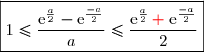
, \le \dfrac{\text e^{\frac {-2x}{ 2} }+\text e^{\frac {-4x}{ 2}}}{2}\quad(\text{voir question 3. a)} ) ,
,![\boxed{\forall\,x\in\;]\,0\;;\;+\infty \,[,\;\text e^{-\frac 3 2 x}\le g(x) \le \dfrac{\text e^{-x}+\text e^{-2x}}{2}}\quad(3)](https://latex.ilemaths.net/latex-0.tex?\boxed{\forall\,x\in\;]\,0\;;\;+\infty \,[,\;\text e^{-\frac 3 2 x}\le g(x) \le \dfrac{\text e^{-x}+\text e^{-2x}}{2}}\quad(3) )
-1}{x}\;.)
![\forall\,x\in\;]\,0\;;\;+\infty \,[\,,\; \\\\\text e^{-\frac 3 2 x}\le g(x) \le \dfrac{\text e^{-x}+\text e^{-2x}}{2}\quad\Longrightarrow\quad\text e^{-\frac 3 2 x}-1\le g(x)-1 \le \dfrac{\text e^{-x}+\text e^{-2x}}{2}-1 \\\overset{ { \white{ . } } } {\phantom{WWWWWWWWWwW}\quad\Longrightarrow\quad\text e^{-\frac 3 2 x}-1\le g(x)-1 \le \dfrac{\text e^{-x}+\text e^{-2x}-2}{2}} \\\overset{ { \white{ . } } } {\phantom{WWWWWWWWWwW}\quad\Longrightarrow\quad\boxed{\dfrac{\text e^{-\frac 3 2 x}-1}{x}\le \dfrac{g(x)-1}{x} \le \dfrac{\text e^{-x}+\text e^{-2x}-2}{2x}}}](https://latex.ilemaths.net/latex-0.tex?\forall\,x\in\;]\,0\;;\;+\infty \,[\,,\; \\\\\text e^{-\frac 3 2 x}\le g(x) \le \dfrac{\text e^{-x}+\text e^{-2x}}{2}\quad\Longrightarrow\quad\text e^{-\frac 3 2 x}-1\le g(x)-1 \le \dfrac{\text e^{-x}+\text e^{-2x}}{2}-1 \\\overset{ { \white{ . } } } {\phantom{WWWWWWWWWwW}\quad\Longrightarrow\quad\text e^{-\frac 3 2 x}-1\le g(x)-1 \le \dfrac{\text e^{-x}+\text e^{-2x}-2}{2}} \\\overset{ { \white{ . } } } {\phantom{WWWWWWWWWwW}\quad\Longrightarrow\quad\boxed{\dfrac{\text e^{-\frac 3 2 x}-1}{x}\le \dfrac{g(x)-1}{x} \le \dfrac{\text e^{-x}+\text e^{-2x}-2}{2x}}} )
\quad\text{où}\;v\text{ est la fonction définie par }:x\to \text e^{-\frac 3 2 x} \\\\\text{Or }v(x)=\text e^{-\frac 3 2 x}\quad\Longrightarrow\quad v'(x)=-\frac 3 2\text e^{-\frac 3 2 x} \\\overset{ { \white{ . } } } {\phantom{WWWWWiW}\quad\Longrightarrow\quad v'(0)=-\frac 3 2\text e^{0}} \\\overset{ { \white{ . } } } {\phantom{WWWWWiW}\quad\Longrightarrow\quad v'(0)=-\dfrac 3 2} \\\\\Longrightarrow\quad\boxed{\lim\limits_{\underset{>}{x\to0}}\,\dfrac{\text e^{-\frac 3 2 x}-1}{x}=-\dfrac 3 2})
 , soit
}{x} \\\phantom{WWWWWWwWWW}=\dfrac 1 2\times\lim\limits_{\underset{>}{x\to0}}\text e^{-2x}\times \lim\limits_{\underset{>}{x\to0}}\,\dfrac{1+\text e^{x}-2\text e^{2x}}{x} \\\phantom{WWWWWWwWWW}=\dfrac 1 2\times\text e^{0}\times \lim\limits_{\underset{>}{x\to0}}\,\dfrac{1+\text e^{x}-2\text e^{2x}}{x} \\\phantom{WWWWWWwWWW}=\dfrac 1 2\times1\times \lim\limits_{\underset{>}{x\to0}}\,\dfrac{1+\text e^{x}-2\text e^{2x}}{x} \\\\\text{D'où }\;\boxed{\dfrac 1 2\times\lim\limits_{\underset{>}{x\to0}}\,\dfrac{\text e^{-2x}+\text e^{-x}-2}{x}=\dfrac 1 2\times\lim\limits_{\underset{>}{x\to0}}\,\dfrac{-2\text e^{2x}+\text e^{x}+1}{x}})
 Déterminons
-(\text e^{x}-1)}{x} \\\phantom{WWWWWWWW}=\lim\limits_{\underset{>}{x\to0}}\,\dfrac{(-2\text e^{x}-1)(\text e^{x}-1)}{x} \\\phantom{WWWWWWWW}=\lim\limits_{\underset{>}{x\to0}}(-2\text e^{x}-1)\times\lim\limits_{\underset{>}{x\to0}}\,\dfrac{\text e^{x}-1}{x} \\\phantom{WWWWWWWW}=(-2\text e^{0}-1)\times\lim\limits_{\underset{>}{x\to0}}\,\dfrac{\text e^{x}-1}{x} \\\phantom{WWWWWWWW}=-3\times\lim\limits_{\underset{>}{x\to0}}\,\dfrac{\text e^{x}-1}{x})
\quad\text{où}\;w\text{ est la fonction définie par }:x\to \text e^{x} \\\\\text{Or }w(x)=\text e^{x}\quad\Longrightarrow\quad w'(x)=\text e^{ x} \\\overset{ { \white{ . } } } {\phantom{WWWWiW}\quad\Longrightarrow\quad w'(0)=\text e^{0}} \\\overset{ { \white{ . } } } {\phantom{WWWWiW}\quad\Longrightarrow\quad w'(0)=1} \\\\\Longrightarrow\quad\boxed{\lim\limits_{\underset{>}{x\to0}}\,\dfrac{-2\text e^{2x}+\text e^{x}+1}{x}=-3\times1=-3})
 \\\\\Longrightarrow\quad\boxed{\lim\limits_{\underset{>}{x\to0}}\,\dfrac{\text e^{-x}+\text e^{-2x}-2}{2x} =-\dfrac 3 2})
-1}{x} \le \dfrac{\text e^{-x}+\text e^{-2x}-2}{2x}\\ \lim\limits_{\underset{>}{x\to0}}\,\dfrac{\text e^{-\frac 3 2 x}-1}{x}=-\dfrac 3 2\phantom{WWWWWWWW}\\ \lim\limits_{\underset{>}{x\to0}}\,\dfrac{\text e^{-x}+\text e^{-2x}-2}{2x} =-\dfrac 3 2\phantom{WWWwWW}\end{matrix}\right.\quad\Longrightarrow\quad\boxed{\lim\limits_{\underset{>}{x\to0}}\,\dfrac{g(x)-1}{x}=-\dfrac 3 2})
=1+\ln\left(\dfrac{1+0}{1-0}\right)=1+\ln1=1+0=1\quad\Longrightarrow\quad\boxed{f(0)=1}\,. } )
![\overset{ { \white{ . } } }{\bullet}{\white{x}}\lim\limits_{\underset{<}{x\to0}}\,f(x)=\lim\limits_{\underset{<}{x\to0}}\,\left[1+\ln\left(\dfrac{1+x}{1-x}\right)\right]=1+\ln\left(\dfrac{1+0}{1-0}\right)=1+\ln1=1 \\\\\phantom{W}\Longrightarrow\quad\boxed{\lim\limits_{\underset{<}{x\to0}}\,f(x)=1}](https://latex.ilemaths.net/latex-0.tex?\overset{ { \white{ . } } }{\bullet}{\white{x}}\lim\limits_{\underset{<}{x\to0}}\,f(x)=\lim\limits_{\underset{<}{x\to0}}\,\left[1+\ln\left(\dfrac{1+x}{1-x}\right)\right]=1+\ln\left(\dfrac{1+0}{1-0}\right)=1+\ln1=1 \\\\\phantom{W}\Longrightarrow\quad\boxed{\lim\limits_{\underset{<}{x\to0}}\,f(x)=1})
=\lim\limits_{\underset{>}{x\to0}}\,\dfrac{\text e^x-1}{x\,\text e^{2x}} \\\phantom{WWWWW}=\lim\limits_{\underset{>}{x\to0}}\,\dfrac{1}{\text e^{2x}}\times\lim\limits_{\underset{>}{x\to0}}\,\dfrac{\text e^x-1}{x} \\\overset{ { \white{ . } } } {\phantom{WWWWW}=\dfrac{1}{\text e^{0}}\times1=1} \\\\\Longrightarrow\quad\boxed{\lim\limits_{\underset{>}{x\to0}}\,f(x)=1})
=1} } )
=f(0)} } )
-f(0)}{x-0}=\lim\limits_{\underset{<}{x\to0}}\,\dfrac{\ln\left(\dfrac{1+x}{1-x}\right)}{x}})

=1+x \\\phantom{\text{Or }\;t=\dfrac{1+x}{1-x}}\quad\Longleftrightarrow\quad t-tx=1+x \\\phantom{vWWWWW}\quad\Longleftrightarrow\quad t-1=tx+x \\\overset{ { \white{ . } } } { \phantom{vWWWWW}\quad\Longleftrightarrow\quad t-1=(t+1)x} \\\overset{ { \white{ . } } } { \phantom{vWWWWW}\quad\Longleftrightarrow\quad x=\dfrac{t-1}{t+1}\quad(t\neq-1)})
\quad\Longleftrightarrow\quad (t\to1))
-f(0)}{x-0}=\lim\limits_{\underset{<}{x\to0}}\,\dfrac{\ln\left(\dfrac{1+x}{1-x}\right)}{x} \\\overset{ { \white{ . } } } {\phantom{WWWWwWW}=\lim\limits_{\underset{<}{t\to1}}\,\dfrac{\ln t}{\frac{t-1}{t+1}} } \\\overset{ { \white{ . } } } {\phantom{WWWWwWW}=\lim\limits_{\underset{<}{t\to1}}\,\dfrac{\ln t}{t-1}\times (t+1) } \\\overset{ { \white{ . } } } {\phantom{WWWWwWW}=\lim\limits_{\underset{<}{t\to1}}\,\dfrac{\ln t}{t-1}\times \lim\limits_{\underset{<}{t\to1}}\,(t+1) })
\quad\text{où}\;m\text{ est la fonction définie par }:x\to \ln x \\\\\phantom{x}\quad\text{Nous savons que }\;m(x)=\ln x\quad\Longrightarrow\quad m'(x)=\dfrac 1 x \\\overset{ { \white{ . } } } {\phantom{WWWWWWWWWxWWWW}\quad\Longrightarrow\quad m'(1)=1} \\\\\Longrightarrow\quad \boxed{\lim\limits_{\underset{<}{t\to1}}\,\dfrac{\ln t}{t-1}=1})
=1+1\quad\Longrightarrow\quad\boxed{\lim\limits_{\underset{<}{t\to1}}\,(t+1)=2})
-f(0)}{x-0}=\lim\limits_{\underset{<}{t\to1}}\,\dfrac{\ln t}{t-1}\times \lim\limits_{\underset{<}{t\to1}}\,(t+1) =1\times2 \\\\\Longrightarrow\quad\boxed{\lim\limits_{\underset{<}{x\to0}}\,\dfrac{f(x)-f(0)}{x-0}=2\in\R})

![\forall\,x\in\;]\,0\;;\;+\infty[,\;f(x)=\dfrac{\text e^x-1}{x\,\text e^{2x}}\quad\Longrightarrow\quad \boxed{\forall\,x\in\;]\,0\;;\;+\infty[,\;f(x)=g(x)}](https://latex.ilemaths.net/latex-0.tex? \forall\,x\in\;]\,0\;;\;+\infty[,\;f(x)=\dfrac{\text e^x-1}{x\,\text e^{2x}}\quad\Longrightarrow\quad \boxed{\forall\,x\in\;]\,0\;;\;+\infty[,\;f(x)=g(x)})
-f(0)}{x-0}=\lim\limits_{\underset{>}{x\to0}}\,\dfrac{g(x)-1}{x}=-\dfrac{3}{2}\quad(\text{voir question 4. b - Partie A)} \\\\\Longrightarrow\quad\boxed{\lim\limits_{\underset{>}{x\to0}}\,\dfrac{f(x)-f(0)}{x-0}=-\dfrac{3}{2}\in\R})

 admet un point anguleux de coordonnées (0 ; 1).
 admet une demi-tangente à gauche de coefficient directeur égal à 2 et une demi-tangente à droite de coefficient directeur égal à
  } ) et
et . } )
![\lim\limits_{x\to-1}f(x)=\lim\limits_{x\to-1}\left[1+\ln\left(\dfrac{1+x}{1-x}\right)\right].](https://latex.ilemaths.net/latex-0.tex?\lim\limits_{x\to-1}f(x)=\lim\limits_{x\to-1}\left[1+\ln\left(\dfrac{1+x}{1-x}\right)\right].)
![\left\lbrace\begin{matrix}\lim\limits_{x\to-1}\left(\dfrac{1+x}{1-x}\right)=0\\\overset{ { \white{ . } } } {\lim\limits_{X\to 0}\ln X=-\infty}\end{matrix}\right.\quad\underset{\left(X=\frac{1+x}{1-x}\right)}{\Longrightarrow}\quad\lim\limits_{x\to-1}\ln\left(\dfrac{1+x}{1-x}\right)=-\infty \\\phantom{WWWWWWxWWW}\quad\Longrightarrow\quad\lim\limits_{x\to-1}\left[1+\ln\left(\dfrac{1+x}{1-x}\right)\right]=-\infty \\\overset{ { \white{ . } } } {\phantom{WWWWWWxWWW}\quad\Longrightarrow\quad\boxed{\lim\limits_{x\to-1}f(x)=-\infty}}](https://latex.ilemaths.net/latex-0.tex?\left\lbrace\begin{matrix}\lim\limits_{x\to-1}\left(\dfrac{1+x}{1-x}\right)=0\\\overset{ { \white{ . } } } {\lim\limits_{X\to 0}\ln X=-\infty}\end{matrix}\right.\quad\underset{\left(X=\frac{1+x}{1-x}\right)}{\Longrightarrow}\quad\lim\limits_{x\to-1}\ln\left(\dfrac{1+x}{1-x}\right)=-\infty \\\phantom{WWWWWWxWWW}\quad\Longrightarrow\quad\lim\limits_{x\to-1}\left[1+\ln\left(\dfrac{1+x}{1-x}\right)\right]=-\infty \\\overset{ { \white{ . } } } {\phantom{WWWWWWxWWW}\quad\Longrightarrow\quad\boxed{\lim\limits_{x\to-1}f(x)=-\infty}})
=\lim\limits_{x\to+\infty}\dfrac{\text e^x-1}{x\,\text e^{2x}}=\lim\limits_{x\to+\infty}g(x)\,.)
![\forall\,x\in\;]\,0\;;\;+\infty \,[,\;\text e^{-\frac 3 2 x}\le g(x) \le \dfrac{\text e^{-x}+\text e^{-2x}}{2}](https://latex.ilemaths.net/latex-0.tex?\forall\,x\in\;]\,0\;;\;+\infty \,[,\;\text e^{-\frac 3 2 x}\le g(x) \le \dfrac{\text e^{-x}+\text e^{-2x}}{2})
 \le \dfrac{\text e^{-x}+\text e^{-2x}}{2}\phantom{WWWW}\\ \lim\limits_{x\to+\infty}\,\text e^{-\frac 3 2 x}=0\phantom{WWWWWWWWWW}\\ \lim\limits_{x\to+\infty}\,\dfrac{\text e^{-x}+\text e^{-2x}}{2}=\dfrac 0 2=0\phantom{WWWwWW}\end{matrix}\right.\quad\Longrightarrow\quad\lim\limits_{x\to+\infty}\,g(x)=0 \\\phantom{WWWWWWWWwWWWWWWWWW}\quad\Longrightarrow\quad\boxed{\lim\limits_{x\to+\infty}\,f(x)=0})
}) sur
sur ![\overset{ { \white{ . } } } {]\,-1\;;\;0 \,[. }](https://latex.ilemaths.net/latex-0.tex?\overset{ { \white{ . } } } {]\,-1\;;\;0 \,[. })
![\forall\,x\in\,]-1\;;\;0\,[,\; f'(x)=\left[1+\ln\left(\dfrac{1+x}{1-x}\right)\right]' \\\phantom{WWWWWWWWW}=0+\dfrac{1}{\dfrac{1+x}{1-x}}\times\left(\dfrac{1+x}{1-x}\right)' \\\overset{ { \white{ . } } } {\phantom{WWWWWWWWW}=\dfrac{1-x}{1+x}\times\dfrac{1\times(1-x)-(1+x)\times(-1)}{(1-x)^2}} \\\overset{ { \white{ . } } } {\phantom{WWWWWWWWW}=\dfrac{1-x}{1+x}\times\dfrac{2}{(1-x)^2}} \\\overset{ { \white{ . } } } {\phantom{WWWWWWWWW}=\dfrac{2}{(1+x)(1-x)}} \\\\\Longrightarrow\boxed{\forall\,x\in\,]-1\;;\;0\,[,\; f'(x)=\dfrac{2}{1-x^2}}](https://latex.ilemaths.net/latex-0.tex?\forall\,x\in\,]-1\;;\;0\,[,\; f'(x)=\left[1+\ln\left(\dfrac{1+x}{1-x}\right)\right]' \\\phantom{WWWWWWWWW}=0+\dfrac{1}{\dfrac{1+x}{1-x}}\times\left(\dfrac{1+x}{1-x}\right)' \\\overset{ { \white{ . } } } {\phantom{WWWWWWWWW}=\dfrac{1-x}{1+x}\times\dfrac{1\times(1-x)-(1+x)\times(-1)}{(1-x)^2}} \\\overset{ { \white{ . } } } {\phantom{WWWWWWWWW}=\dfrac{1-x}{1+x}\times\dfrac{2}{(1-x)^2}} \\\overset{ { \white{ . } } } {\phantom{WWWWWWWWW}=\dfrac{2}{(1+x)(1-x)}} \\\\\Longrightarrow\boxed{\forall\,x\in\,]-1\;;\;0\,[,\; f'(x)=\dfrac{2}{1-x^2}})
![\overset{ { \white{ . } } } {]\,0\;;\;+\infty \,[. }](https://latex.ilemaths.net/latex-0.tex?\overset{ { \white{ . } } } {]\,0\;;\;+\infty \,[. })
![\overset{ { \white{ . } } } { \forall\,x\in\;]\,0\;;\;+\infty\,[\,,f(x)=g(x).}](https://latex.ilemaths.net/latex-0.tex?\overset{ { \white{ . } } } { \forall\,x\in\;]\,0\;;\;+\infty\,[\,,f(x)=g(x).} )
![\overset{ { \white{ . } } } { \forall\,x\in\;]\,0\;;\;+\infty\,[\,,f'(x)=g'(x).}](https://latex.ilemaths.net/latex-0.tex?\overset{ { \white{ . } } } { \forall\,x\in\;]\,0\;;\;+\infty\,[\,,f'(x)=g'(x).} )
![\overset{ { \white{ . } } } {\forall\,x\in\,]\,0\;;\;+\infty\,[,\;g'(x)=\text e^{-2x}\left[\dfrac{1+2x-(x+1)\,\text e^{x}}{x^2}\right]}](https://latex.ilemaths.net/latex-0.tex?\overset{ { \white{ . } } } {\forall\,x\in\,]\,0\;;\;+\infty\,[,\;g'(x)=\text e^{-2x}\left[\dfrac{1+2x-(x+1)\,\text e^{x}}{x^2}\right]})
![\overset{ { \white{ . } } } {\boxed{\forall\,x\in\,]\,0\;;\;+\infty\,[,\;f'(x)=\text e^{-2x}\left[\dfrac{1+2x-(x+1)\,\text e^{x}}{x^2}\right]}}](https://latex.ilemaths.net/latex-0.tex?\overset{ { \white{ . } } } {\boxed{\forall\,x\in\,]\,0\;;\;+\infty\,[,\;f'(x)=\text e^{-2x}\left[\dfrac{1+2x-(x+1)\,\text e^{x}}{x^2}\right]}})
 sur
sur ![x\in\,]-1\;;\;0\,[\quad\Longrightarrow\quad-1<x<0 \\\overset{ { \white{ . } } } {\phantom{x\in]-1\;;\;0\,[}\quad\Longrightarrow\quad0<x^2<1} \\\overset{ { \white{ . } } } {\phantom{x\in]-1\;;\;0\,[}\quad\Longrightarrow\quad-1<-x^2<0} \\\overset{ { \white{ . } } } {\phantom{x\in]-1\;;\;0\,[}\quad\Longrightarrow\quad0<1-x^2<1}](https://latex.ilemaths.net/latex-0.tex?x\in\,]-1\;;\;0\,[\quad\Longrightarrow\quad-1<x<0 \\\overset{ { \white{ . } } } {\phantom{x\in]-1\;;\;0\,[}\quad\Longrightarrow\quad0<x^2<1} \\\overset{ { \white{ . } } } {\phantom{x\in]-1\;;\;0\,[}\quad\Longrightarrow\quad-1<-x^2<0} \\\overset{ { \white{ . } } } {\phantom{x\in]-1\;;\;0\,[}\quad\Longrightarrow\quad0<1-x^2<1})
![\\\overset{ { \white{ . } } } {\phantom{x\in]-1\;;\;0\,[}\quad\Longrightarrow\quad0<\dfrac{2}{1-x^2}} \\\overset{ { \white{ . } } } {\phantom{x\in]-1\;;\;0\,[}\quad\Longrightarrow\quad0<f'(x)} \\\\\Longrightarrow\quad\boxed{\forall\,x\in\,]-1\;;\;0\,[\,,\;f'(x)>0}](https://latex.ilemaths.net/latex-0.tex?\\\overset{ { \white{ . } } } {\phantom{x\in]-1\;;\;0\,[}\quad\Longrightarrow\quad0<\dfrac{2}{1-x^2}} \\\overset{ { \white{ . } } } {\phantom{x\in]-1\;;\;0\,[}\quad\Longrightarrow\quad0<f'(x)} \\\\\Longrightarrow\quad\boxed{\forall\,x\in\,]-1\;;\;0\,[\,,\;f'(x)>0})

&&+&\phantom{xi}(2)||(-\frac32)&-&\\&&&||&&\\\hline &&&1&&\\f(x)&&\nearrow&&\searrow&\\&-\infty&&&&0\\\hline \end{array})
. })
 la partie du plan délimitée par la courbe
  et
et 
} }) en cm2.
en cm2.![\text e^{-\frac 3 2 x}\le g(x) \le \dfrac{\text e^{-x}+\text e^{-2x}}{2}\quad\Longrightarrow\quad\displaystyle\int_{0}^{1}\text e^{-\frac 3 2 x}\text{ d}x\le \displaystyle\int_{0}^{1}g(x)\text{ d}x \le \displaystyle\int_{0}^{1}\dfrac{\text e^{-x}+\text e^{-2x}}{2}\text{ d}x \\\\\phantom{WWWWWWWWWWW}\quad\Longrightarrow\quad\displaystyle\int_{0}^{1}\text e^{-\frac 3 2 x}\text{ d}x\le \displaystyle\int_{0}^{1}g(x)\text{ d}x \le \dfrac 1 2\displaystyle\int_{0}^{1}(\text e^{-x}+\text e^{-2x})\text{ d}x \\\\\phantom{WWWWWWWWWWW}\quad\Longrightarrow\quad-\dfrac 2 3\left[\text e^{-\frac 3 2 x}\right]_{0}^{1}\le \mathscr{A(D)} \le \dfrac 1 2\left[-\text e^{-x}-\dfrac 1 2\,\text e^{-2x}\right]_{0}^{1} \\\\\phantom{WWWWWWWWWWW}\quad\Longrightarrow\quad-\dfrac 2 3\left[\text e^{-\frac 3 2 }-\text e^{0}\right]\le \mathscr{A(D)} \le \dfrac 1 2\left[-(\text e^{-1}-\text e^{0})-\dfrac 1 2\,(\text e^{-2}-\text e^{0})\right]](https://latex.ilemaths.net/latex-0.tex?\text e^{-\frac 3 2 x}\le g(x) \le \dfrac{\text e^{-x}+\text e^{-2x}}{2}\quad\Longrightarrow\quad\displaystyle\int_{0}^{1}\text e^{-\frac 3 2 x}\text{ d}x\le \displaystyle\int_{0}^{1}g(x)\text{ d}x \le \displaystyle\int_{0}^{1}\dfrac{\text e^{-x}+\text e^{-2x}}{2}\text{ d}x \\\\\phantom{WWWWWWWWWWW}\quad\Longrightarrow\quad\displaystyle\int_{0}^{1}\text e^{-\frac 3 2 x}\text{ d}x\le \displaystyle\int_{0}^{1}g(x)\text{ d}x \le \dfrac 1 2\displaystyle\int_{0}^{1}(\text e^{-x}+\text e^{-2x})\text{ d}x \\\\\phantom{WWWWWWWWWWW}\quad\Longrightarrow\quad-\dfrac 2 3\left[\text e^{-\frac 3 2 x}\right]_{0}^{1}\le \mathscr{A(D)} \le \dfrac 1 2\left[-\text e^{-x}-\dfrac 1 2\,\text e^{-2x}\right]_{0}^{1} \\\\\phantom{WWWWWWWWWWW}\quad\Longrightarrow\quad-\dfrac 2 3\left[\text e^{-\frac 3 2 }-\text e^{0}\right]\le \mathscr{A(D)} \le \dfrac 1 2\left[-(\text e^{-1}-\text e^{0})-\dfrac 1 2\,(\text e^{-2}-\text e^{0})\right])
![\\\\\phantom{WWWWWWWWWWW}\quad\Longrightarrow\quad-\dfrac 2 3\left[\text e^{-\frac 3 2 }-1\right]\le \mathscr{A(D)} \le \dfrac 1 2\left[-(\text e^{-1}-1)-\dfrac 1 2\,(\text e^{-2}-1)\right] \\\\\phantom{WWWWWWWWWWW}\quad\Longrightarrow\quad-\dfrac 2 3\left[\text e^{-\frac 3 2 }-1\right]\le \mathscr{A(D)} \le \dfrac 1 2\left[-\text e^{-1}-\dfrac 1 2\,\text e^{-2}+\dfrac 32\right] \\\\\text{Or }\;\left\lbrace\begin{matrix}-\dfrac 2 3\left[\text e^{-\frac 3 2 }-1\right]\approx0,518\;\text{u.a.}\phantom{XXXX} \\\\\dfrac 1 2\left[-\text e^{-1}-\dfrac 1 2\,\text e^{-2}+\dfrac 32\right]\approx0,532\;\text{u.a.}\end{matrix}\right. \\\\\text{D'où }\quad\boxed{0,518\;\text{u.a.}\le\mathscr{A(D)} \le0,532\;\text{u.a.}}](https://latex.ilemaths.net/latex-0.tex?\\\\\phantom{WWWWWWWWWWW}\quad\Longrightarrow\quad-\dfrac 2 3\left[\text e^{-\frac 3 2 }-1\right]\le \mathscr{A(D)} \le \dfrac 1 2\left[-(\text e^{-1}-1)-\dfrac 1 2\,(\text e^{-2}-1)\right] \\\\\phantom{WWWWWWWWWWW}\quad\Longrightarrow\quad-\dfrac 2 3\left[\text e^{-\frac 3 2 }-1\right]\le \mathscr{A(D)} \le \dfrac 1 2\left[-\text e^{-1}-\dfrac 1 2\,\text e^{-2}+\dfrac 32\right] \\\\\text{Or }\;\left\lbrace\begin{matrix}-\dfrac 2 3\left[\text e^{-\frac 3 2 }-1\right]\approx0,518\;\text{u.a.}\phantom{XXXX} \\\\\dfrac 1 2\left[-\text e^{-1}-\dfrac 1 2\,\text e^{-2}+\dfrac 32\right]\approx0,532\;\text{u.a.}\end{matrix}\right. \\\\\text{D'où }\quad\boxed{0,518\;\text{u.a.}\le\mathscr{A(D)} \le0,532\;\text{u.a.}})
} \le0,532\times 9\;\text{cm}^2} )
} \le4,79\;\text{cm}^2}} ) Publié par malou/Panter
le
Publié par malou/Panter
le
 Voir la correction
 forum de terminale