Seules les calculatrices scientifiques non graphiques sont autorisées.
2 points
exercice 1
Écris sur ta feuille de copie, le numéro de chaque proposition suivi de Vrai si la proposition est vraie ou de Faux si
la proposition est fausse.
2 points
exercice 2
Pour chacun des énoncés du tableau ci-dessous, les informations des lignes A, B, C et D permettent d'obtenir quatre affirmations dont une seule est vraie.
Écris, sur ta feuille de copie, le numéro de l'énoncé suivi de la lettre de la ligne qui donne l'affirmation vraie.
3 points
exercice 3
Des scientifiques participent à un séminaire sur le thème : "Le réchauffement climatique et ses conséquences sur les économies des pays".
Une enquête organisée par un organisme international a révélé que 75% des scientifiques croient au réchauffement climatique et parmi
ceux-ci, il y a des écologistes.
Selon cette enquête :
la probabilité qu'un scientifique qui croit au réchauffement climatique soit un écologiste est 0,6 ;
la probabilité qu'un scientifique qui ne croit pas au réchauffement climatique ne soit
pas un écologiste est 0,08.
On choisit un scientifique au hasard ayant participé au séminaire.
On désigne par : R l'évènement : "Le scientifique interrogé croit au réchauffement climatique" ; E l'évènement : "Le scientifique interrogé est un écologiste".
1. a. Traduis cette situation à l'aide d'un arbre pondéré. b. Donne les probabilités suivantes : 2. a. Calcule b. Justifie que 3. a. Justifie que la probabilité qu'un scientifique interrogé soit un écologiste est 0,68. b. Un scientifique interrogé est un écologiste. Calcule la probabilité qu'il ne croit pas au réchauffement climatique. (Tu donneras l'arrondi
d'ordre 2 du résultat ).
4 points
exercice 4
Soit m un nombre réel et la fonction de R vers R, définie par :
On note l'ensemble de définition de et on désigne par sa courbe représentative
dans le plan muni d'un repère (O; I; J).
On désigne par la droite d'équation :
1. Justifie que : a. Si alors b. Si alors 2. On suppose que est dérivable sur pour tout nombre réel m. a. Justifie que pour tout x de b. Justifie que pour est strictement croissante sur R. c. Justifie que pour est strictement croissante sur 3. a. Démontre que pour tout nombre réel est une bijection sur b. Établis que pour tout nombre réel m et pour tout nombre réel x élément
de on a : c. Déduis de la question précédente, une méthode de construction de dans
le même repère que 4. On suppose que m et p sont des nombres réels strictement positifs. a. Justifie que est l'image de par la translation T de vecteur
b. Détermine la translation T' qui transforme en
4 points
exercice 5
On considère l'équation (E) : où les inconnues x et y appartiennent à Z.
1. a. Démontrer que si le couple est une solution de (E), alors est pair. b. Détermine les valeurs possibles de 2. a. Vérifie que le couple (1 ; 2) est une solution de (E). b. Résous l'équation (E).
3. Détermine l'ensemble des couples (x, y) solutions de (E) tels que x et y soient premiers entre eux.
4. sont deux écritures du même entier naturel p
respectivement en base 3 et en base 4.
a. Justifie que 3c + 2 est multiple de 4. b. Déduis-en que c est égal à 2. c. Détermine les valeurs de a et b. (Tu pourras utiliser 2. b.). d. Écris p dans le système décimal.
5 points
exercice 6
Une étudiante en histoire ancienne veut rédiger son mémoire de Master 2. Au cours de ses recherches, elle décide de déterminer l'âge
d'un fragment d'os découvert par les archéologues.
L'information dont elle dispose est que le fragment découvert a une teneur en carbone 14 égale à 70% de celle d'un fragment d'os
actuel de même masse pris comme témoin.
Au cours de sa formation, elle a appris que : Si t est l'âge en années de l'os découvert, alors la quantité restante de carbone 14 dans le fragment
d'os est où est une fonction de La dérivée de la fonction est égale au produit de par l'opposé de
la constante radioactive de carbone 14, notée La quantité de carbone 14 d'un organisme vivant commence à diminuer à partir de la mort de cet
organisme à l'instant t égal à 0.
N'ayant pas suffisamment de connaissances pour exploiter ces données, elle te sollicite.
A l'aide d'une production argumentée basée sur tes connaissances mathématiques, réponds à la préoccupation de l'étudiante.
Proposition n°1 Dans l'espace muni d'un repère orthonormé , si est le plan d'équation cartésienne : , alors un vecteur normal à est : Proposition vraie.
En effet, un vecteur normal à est ou un vecteur colinéaire à .
Or car
Donc un vecteur normal à est :
Par conséquent, la proposition n° 1 est vraie.
Proposition n°2 Le plan est muni d'un repère orthonormé (O,I,J). L'ellipse d'équation réduite : de demi distance focale a pour foyers et tels que : et Proposition fausse.
En effet, puisque 9 < 16, l'ellipse a pour foyers et tels que : et
Proposition n°3 Une corrélation linéaire entre deux caractères et d'une série statistique double est forte lorsque le coefficient de corrélation linéaire est tel que : Proposition fausse.
En effet, il y a une forte corrélation linéaire entre les deux caractères et si est proche de 1, soit en pratique si ou
Proposition n°4 Soit et deux points distincts du plan. La composée est une rotation d'angle Proposition vraie.
En effet, la composée d'une rotation d'angle et d'une translation est une rotation d'angle .
2 points
exercice 2
Énoncé n°1 : Réponse C. La suite de terme général : a pour limite
En effet, et si alors
Énoncé n°2 : Réponse D.
est un carré de centre tel que le triplet soit de sens direct. et sont les milieux respectifs des segments et
La composée est la symétrie glissée d'axe et de vecteur
En effet, soit
La forme réduite de la symétrie glissée d'axe et de vecteur est
D'où soit soit
Énoncé n°3 : Réponse A.
On admet que :
La fonction définie sur [0 ; 1] par : est telle que :
En effet, nous savons que
Dès lors,
Énoncé n°4 : Réponse A.
Dans le plan rapporté à un repère orthonormé (O, I, J), on donne les points A, B et C d'affixes respectives : 2 ; 2+2i et 2i.
La similitude directe de centre A qui transforme B en C a pour angle et pour rapport et
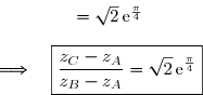
En effet, écrivons sous forme exponentielle.
Dès lors,
le rapport de la similitude est
l'angle de la similitude est
3 points
exercice 3
Une enquête organisée par un organisme international a révélé que 75% des scientifiques croient au réchauffement climatique et parmi ceux-ci, il y a des écologistes.
Selon cette enquête : la probabilité qu'un scientifique qui croit au réchauffement climatique soit un écologiste est 0,6 ; la probabilité qu'un scientifique qui ne croit pas au réchauffement climatique ne soit pas un écologiste est 0,08.
On choisit un scientifique au hasard ayant participé au séminaire.
On désigne par : R l'événement : ''Le scientifique interrogé croit au réchauffement climatique'' ; E l'événement : ''Le scientifique interrogé est un écologiste''.
1. a) Construisons un arbre pondéré traduisant la situation.
1. b) En utilisant l'arbre pondéré, nous obtenons :
2. a)
2. b) Calculons
3. a) Nous devons déterminer
Les événements et forment une partition de l'univers.
En utilisant la formule des probabilités totales, nous obtenons :
3. b) Un scientifique interrogé est un écologiste. Calculons la probabilité qu'il ne croie pas au réchauffement climatique.
Nous devons déterminer
D'où, la probabilité qu'un scientifique écologiste ne croie pas au réchauffement climatique est environ égale à 0,34.
4 points
exercice 4
Soit un nombre réel et la fonction de vers , définie par :
On note l'ensemble de définition de et on désigne par sa courbe représentative dans le plan muni d'un repère (O; I; J).
On désigne par la droite d'équation :
1. Déterminons
1. a)Premier cas :
Par conséquent, si alors
1. b)Deuxième cas :
Par conséquent, si alors
2. On suppose que est dérivable sur pour tout nombre réel
2. a) Déterminons l'expression algébrique de
Pour tout
2. b) Étudions la croissance de pour
L'exponentielle est strictement positive pour tout réel
Donc le signe de est le signe de :
Par conséquent, pour est strictement croissante sur
2. c) Étudions la croissance de sur pour
L'exponentielle est strictement positive pour tout réel
Donc le signe de est le signe de :
Par conséquent, pour est strictement croissante sur
3. a) Démontrons que pour tout nombre réel est une bijection sur
Premier cas :
Dans ce cas, la fonction de vers , définie par :
La fonction est continue et strictement croissante sur
Il s'ensuit que réalise une bijection de sur
Deuxième cas :
La fonction est continue et strictement croissante sur
Il s'ensuit que réalise une bijection de sur
Déterminons (non demandé dans l'énoncé )
Calculons
Or la constante 1 est insignifiante comparée à quand tend vers
Nous obtenons ainsi :
Calculons
D'où
Par conséquent, réalise une bijection de sur
Troisième cas :
La fonction est continue et strictement croissante sur
Il s'ensuit que réalise une bijection de sur
Déterminons (non demandé dans l'énoncé ).
Calculons
Dès lors,
D'où
Calculons
D'où
Par conséquent, réalise une bijection de sur
3. b) Nous devons établir que pour tout nombre réel et pour tout nombre réel élément de on a :
Montrons que pour tout nombre réel et pour tout nombre réel élément de on a :
En effet, pour tout et pour tout
Par conséquent,
3. c) Nous déduisons de la question précédente que est le symétrique de par rapport à la droite
4. On suppose que et sont des nombres réels strictement positifs.
4. a) Nous devons justifier que est l'image de par la translation de vecteur
Montrons donc que
En effet,
Nous obtenons alors :
Par conséquent, l'image de par la translation de vecteur est
4. b) Déterminons la translation qui transforme en
Nous déduisons de la question précédente que :
est l'image de par la translation de vecteur est l'image de par la translation de vecteur
Dès lors, est l'image de par la translation de vecteur
4 points
exercice 5
On considère l'équation où les inconnues et appartiennent à
1. a) Démontrons que si le couple est une solution de , alors est pair.
Le couple est une solution de
Donc nous obtenons :
Il s'ensuit que s'écrit sous la forme avec entier.
Par conséquent, est pair.
1. b) Déterminons les valeurs possibles de
Si est impair, alors Si est pair, alors
Donc
2. a) Le couple (1 ; 2) est une solution de car
2. b) Résolvons l'équation
L'équation équivaut à
Par conséquent, l'ensemble des solutions de l'équation est
3. Déterminons l'ensemble des couples solutions de tels que et soient premiers entre eux.
Nous savons que est pair.
Pour que et soient premiers entre eux, il faut que soit un nombre impair, soit de la forme où
Donc l'ensemble des couples solutions de tels que et soient premiers entre eux est soit
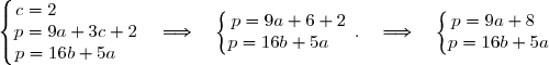
4. sont deux écritures du même entier naturel respectivement en base 3 et en base 4.
4. a) Montrons que est multiple de 4.
Dès lors, par identification, nous obtenons :
soit
soit
Par conséquent, est multiple de 4.
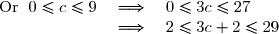
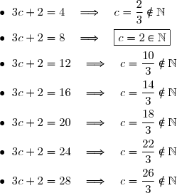
4. b) Nous savons que est multiple de 4.
Nous savons donc que est nombre entier multiple de 4 compris entre 2 et 29.
Donnons comme valeurs à les multiples de 4 compris entre 2 et 29.
Nous en déduisons que
4. c) Déterminons les valeurs de et de
D'où
soit
soit
Nous devons donc déterminer les valeurs entières de et de comprises entre 0 et 9 vérifiant l'équation dont les solutions sont les couples
Nous avons montré dans la question 2. b) que l'ensemble des solutions de l'équation est
Si alors
Donc et
Si alors
Donc et
Les autres valeurs de rendent le problème impossible.
Par conséquent, nous obtenons : ou
5. Écrivons dans le système décimal.
Premier cas :
ou
Second cas :
ou
5 points
exercice 6
Les données du problème nous conduisent à résoudre l'équation différentielle
Les solutions de l'équation différentielle sont les fonctions de la forme
De plus,
Or
Nous en déduisons que
Nous savons que le fragment découvert a une teneur en carbone 14 égale à 70% de celle d'un fragment d'os actuel de même masse pris comme témoin.
Nous avons donc :
Il s'ensuit que
Dès lors,
D'où
Par conséquent, l'âge du fragment d'os découvert par les archéologues est d'environ 2866 ans.
Publié par malou
le
ceci n'est qu'un extrait
Pour visualiser la totalité des cours vous devez vous inscrire / connecter (GRATUIT) Inscription Gratuitese connecter
Merci à Hiphigenie / malou pour avoir contribué à l'élaboration de cette fiche
Désolé, votre version d'Internet Explorer est plus que périmée ! Merci de le mettre à jour ou de télécharger Firefox ou Google Chrome pour utiliser le site. Votre ordinateur vous remerciera !
 la probabilité qu'un scientifique qui croit au réchauffement climatique soit un écologiste est 0,6 ;
 b. Donne les probabilités suivantes :
  ; P_{\overline R} (\overline E) ; P_R(E).)
.)
=0,23.)
 Calcule la probabilité qu'il ne croit pas au réchauffement climatique. (Tu donneras l'arrondi
d'ordre 2 du résultat ).
Calcule la probabilité qu'il ne croit pas au réchauffement climatique. (Tu donneras l'arrondi
d'ordre 2 du résultat ). la fonction de R vers R, définie par :
 =x+\ln (1-m\text e ^{-x}).)
 l'ensemble de définition de
 ) sa courbe représentative
dans le plan muni d'un repère (O; I; J).
sa courbe représentative
dans le plan muni d'un repère (O; I; J).) la droite d'équation :
la droite d'équation : 
 a. Si
a. Si  alors
alors 
 alors
alors ![\text D_m =]\ln (m) ;+\infty[.](https://latex.ilemaths.net/latex-0.tex?\text D_m =]\ln (m) ;+\infty[.)
=\dfrac{\text e^x}{\text e ^x-m})
 est strictement croissante sur R.
 est strictement croissante sur
 ![]\ln (m) ;+\infty[.](https://latex.ilemaths.net/latex-0.tex?]\ln (m) ;+\infty[.)
 est une bijection sur
, ) on a :
on a : =f_{-m}(x).)
) dans
le même repère que
dans
le même repère que .)
) est l'image de
est l'image de ) par la translation T de vecteur
par la translation T de vecteur
\,;\,\ln (p) ).)
 où les inconnues x et y appartiennent à Z.
) est une solution de (E), alors
est une solution de (E), alors  est pair.
.)
 sont deux écritures du même entier naturel p
respectivement en base 3 et en base 4.
sont deux écritures du même entier naturel p
respectivement en base 3 et en base 4.
 Si t est l'âge en années de l'os découvert, alors la quantité restante de carbone 14 dans le fragment
d'os est
Si t est l'âge en années de l'os découvert, alors la quantité restante de carbone 14 dans le fragment
d'os est ) où
où  est une fonction de
 de la fonction
 .)
 de carbone 14 d'un organisme vivant commence à diminuer à partir de la mort de cet
organisme à l'instant t égal à 0.
de carbone 14 d'un organisme vivant commence à diminuer à partir de la mort de cet
organisme à l'instant t égal à 0.
 }) , si
, si  }) est le plan d'équation cartésienne :
est le plan d'équation cartésienne :  , alors un vecteur normal à
 . })
:2x+3y+4z-8=0 }) est
est  }) ou un vecteur colinéaire à
ou un vecteur colinéaire à  .
. car
car =\dfrac12\,(2\;;\;3\;;\;4). })
 de demi distance focale
  a pour foyers
  et
et  tels que :
  }) et
et . })
 et
et  tels que :
  }) et
et . })
 et
et  d'une série statistique double est forte lorsque le coefficient de corrélation linéaire
  est tel que :
 est proche de 1, soit en pratique si
  ou
ou 
 et
et  deux points distincts du plan. La composée
 }\circ t_{\overrightarrow{AB}} }) est une rotation d'angle
est une rotation d'angle 
 et d'une translation est une rotation d'angle
 _{n\in\N} }) de terme général :
de terme général : ^n }) a pour limite
a pour limite 
 et si
et si  alors
alors 
 est un carré de centre
  tel que le triplet
  }) soit de sens direct.
soit de sens direct. et
et  sont les milieux respectifs des segments
 ![\overset{ { \white{ . } } } { [QR] }](https://latex.ilemaths.net/latex-0.tex?\overset{ { \white{ . } } } { [QR] }) et
et ![\overset{ { \white{ . } } } { [RS]. }](https://latex.ilemaths.net/latex-0.tex?\overset{ { \white{ . } } } { [RS]. })
}\circ S_{(QR)} }) est la symétrie glissée d'axe
est la symétrie glissée d'axe  }) et de vecteur
et de vecteur 
}\circ S_{(QR)}.})
 d'axe
d'axe  est
est }\circ t_{\vec u}=t_{\vec u}\circ S_{(IJ)}}\,. })
}(Q)={\red{Q}}\\r_{(O;\frac{\pi}{2})}({\red{Q}})=R\end{matrix}\right.\quad\Longrightarrow\quad \left(r_{(O;\frac{\pi}{2})}\circ S_{(QR)}\right)(Q)=R \\\phantom{WWWWWWWW}\quad\Longrightarrow\quad \boxed{f(Q)=R} \\\\ \overset{ { \phantom{ . } } }{\bullet}{\white{x}} \left\lbrace\begin{matrix}S_{(QR)}(R)={\red{R}}\\r_{(O;\frac{\pi}{2})}({\red{R}})=S\end{matrix}\right.\quad\Longrightarrow\quad \left(r_{(O;\frac{\pi}{2})}\circ S_{(QR)}\right)(R)=S \\\phantom{WWWWWWWW}\quad\Longrightarrow\quad \boxed{f(R)=S })
(Q)=f(f(Q))\\\phantom{WWw}=f(R)\\\phantom{uw}=S\\f\circ f=t_{\vec u}\circ S_{(IJ)}\circ S_{(IJ)}\circ t_{\vec u}\\=t_{\vec u}\circ t_{\vec u}\phantom{WWWi}\\=t_{2\vec u}\phantom{WwWWW} \end{matrix}\right.\quad\Longrightarrow\quad \boxed{t_{2\vec u}(Q)=S })
 soit
soit  soit
soit 
![\overset{ { \white{ . } } } { \forall\,x\in[0\;;\;1], \; \dfrac12\le\dfrac{1}{1+x^2}\le1. }](https://latex.ilemaths.net/latex-0.tex?\overset{ { \white{ . } } } { \forall\,x\in[0\;;\;1], \; \dfrac12\le\dfrac{1}{1+x^2}\le1. })
=\displaystyle\int_1^x\dfrac{1}{1+t^2}\,\text{d}t }) est telle que :
est telle que : \le \dfrac x2-\dfrac12}}\,. })
![\overset{ { \white{ . } } } { \forall\,t\in[0\;;\;1], \; \dfrac12\le\dfrac{1}{1+t^2}\le1. }](https://latex.ilemaths.net/latex-0.tex?\overset{ { \white{ . } } } { \forall\,t\in[0\;;\;1], \; \dfrac12\le\dfrac{1}{1+t^2}\le1. })
![\overset{ { \white{ . } } } {\forall\,x\in[0\;;\;1], \; }](https://latex.ilemaths.net/latex-0.tex?\overset{ { \white{ . } } } {\forall\,x\in[0\;;\;1], \; })
![\displaystyle\int_x^1\dfrac12\,\text{d}t\le\displaystyle\int_x^1\dfrac{1}{1+t^2}\,\text{d}t\le\displaystyle\int_x^11\,\text{d}t \quad\Longrightarrow\quad \left[\overset{}{\dfrac t2}\right]_x^1\le\displaystyle\int_x^1\dfrac{1}{1+t^2}\,\text{d}t\le\left[\overset{\phantom{o}}{t}\right]_x^1 \\\overset{ { \white{ . } } } {\phantom{WxWWWWWWWWWW}\quad\Longrightarrow\quad \dfrac 12-\dfrac x2\le-\displaystyle\int_1^x\dfrac{1}{1+t^2}\,\text{d}t\le1-x} \\\overset{ { \white{ . } } } {\phantom{WxWWWWWWWWWW}\quad\Longrightarrow\quad \dfrac 12-\dfrac x2\le-F(x)\le1-x} \\\overset{ { \white{ . } } } {\phantom{WxWWWWWWWWWW}\quad\Longrightarrow\quad \boxed{x-1\le F(x)\le\dfrac x2-\dfrac12}}](https://latex.ilemaths.net/latex-0.tex?\displaystyle\int_x^1\dfrac12\,\text{d}t\le\displaystyle\int_x^1\dfrac{1}{1+t^2}\,\text{d}t\le\displaystyle\int_x^11\,\text{d}t \quad\Longrightarrow\quad \left[\overset{}{\dfrac t2}\right]_x^1\le\displaystyle\int_x^1\dfrac{1}{1+t^2}\,\text{d}t\le\left[\overset{\phantom{o}}{t}\right]_x^1 \\\overset{ { \white{ . } } } {\phantom{WxWWWWWWWWWW}\quad\Longrightarrow\quad \dfrac 12-\dfrac x2\le-\displaystyle\int_1^x\dfrac{1}{1+t^2}\,\text{d}t\le1-x} \\\overset{ { \white{ . } } } {\phantom{WxWWWWWWWWWW}\quad\Longrightarrow\quad \dfrac 12-\dfrac x2\le-F(x)\le1-x} \\\overset{ { \white{ . } } } {\phantom{WxWWWWWWWWWW}\quad\Longrightarrow\quad \boxed{x-1\le F(x)\le\dfrac x2-\dfrac12}})
 et
et 
 sous forme exponentielle.
}{2\text i}} \\\overset{ { \white{ . } } } {\phantom{WWWw}=1+\text i})
 le rapport de la similitude est
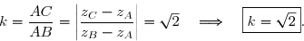
=\arg\left(\dfrac{z_C-z_A}{z_B-z_A}\right)=\dfrac{\pi}{4}\quad\Longrightarrow\quad \boxed{\theta=\dfrac{\pi }{4}}.})
 =0,75 \\\overset{ { \white{ . } } } {P_{\overline R} (\overline E)=0,08} \\\overset{ { \white{ . } } } {P_R(E)=0,6}\end{matrix}\right. })
=1-0,6\quad\Longrightarrow\quad \boxed{P_R(\overline E)=0,4}\,. })
. })
=P(\overline R)\times P_{\overline R}(E) \\\overset{ { \white{ . } } } {\phantom{ P(\overline R\cap E)}=0,25\times 0,92} \\\overset{ { \white{ . } } } {\phantom{ P(\overline R\cap E)}=0,23} \\\\\Longrightarrow\quad\boxed{P(\overline R\cap E)=0,23})
. })
 et
et  forment une partition de l'univers.
=P(R\cap E)+P(\overline{R}\cap E) \\\overset{ { \white{ . } } } {\phantom{P(D)}=P(R)\times P_R(E)+0,23} \\\overset{ { \white{ . } } } {\phantom{P(D)}=0,75\times0,6+0,23} \\\overset{ { \white{ . } } } {\phantom{P(D)}=0,68} \\\\\Longrightarrow\boxed{P(E)=0,68})
.})
=\dfrac{P(\overline{R}\cap E)}{P(E)}=\dfrac{0,23}{0,68}\approx0,34 \\\\\Longrightarrow\boxed{P_E(\overline{R})\approx0,34})
 un nombre réel et
  la fonction de
  vers
vers =x+\ln (1-m\text e ^{-x}). })
 l'ensemble de définition de
  }) sa courbe représentative dans le plan muni d'un repère (O; I; J).
sa courbe représentative dans le plan muni d'un repère (O; I; J). }) la droite d'équation :
la droite d'équation : 
\in\R\quad\Longleftrightarrow\quad \boxed{1-m\text e ^{-x}>0.} })

 \\\overset{ { \white{ . } } } { \phantom{\forall\,x\in\R,\;\text e^{-x}>0}\quad\Longrightarrow\quad -m\text e^{-x}\ge0} \\\overset{ { \white{ . } } } { \phantom{\forall\,x\in\R,\;\text e^{-x}>0}\quad\Longrightarrow\quad 1-m\text e^{-x}\ge1>0} \\\overset{ { \white{ . } } } { \phantom{\forall\,x\in\R,\;\text e^{-x}>0}\quad\Longrightarrow\quad 1-m\text e^{-x}>0} \\\\\Longrightarrow\boxed{\text{Si }m\le0,\;\text{alors }\forall\,x\in\R,\;1-m\text e^{-x}>0})
 alors
alors 

} \\\overset{ { \white{ . } } } {\phantom{1-m\text e^{-x}>0}\quad\Longleftrightarrow\quad -x<-\ln\left(m\right)})
} \\\\\Longrightarrow\boxed{\text{Si }m>0,\;\text{alors }1-m\text e^{-x}>0\quad\Longleftrightarrow\quad x>\ln\left(m\right)})
 alors
alors ![\overset{ { \white{ . } } } { \text D_m =\,]\ln(m)\;;\;+\infty[. }](https://latex.ilemaths.net/latex-0.tex?\overset{ { \white{ . } } } { \text D_m =\,]\ln(m)\;;\;+\infty[. })

 .} )

=\Big(x+\ln (1-m\text e ^{-x})\Big)' \\\overset{ { \white{ . } } } { \phantom{f'_m(x)}=1+\dfrac{(1-m\text e ^{-x})'}{1-m\text e ^{-x} }} \\\overset{ { \white{ . } } } { \phantom{f'_m(x)}=1+\dfrac{m\text e ^{-x}}{1-m\text e ^{-x} }} \\\overset{ { \white{ . } } } { \phantom{f'_m(x)}=\dfrac{1-m\text e ^{-x} +m\text e ^{-x}}{1-m\text e ^{-x} }})
}=\dfrac{1}{1-m\text e ^{-x} }} \\\overset{ { \white{ . } } } { \phantom{f'_m(x)}=\dfrac{1\times \text e^x}{(1-m\text e ^{-x})\times \text e^x }} \\\overset{ { \white{ . } } } { \phantom{f'_m(x)}=\dfrac{\text e^x}{\text e^x-m }} \\\\\Longrightarrow\quad\boxed{\forall\,x\in D_m,\;f'_m(x)=\dfrac{\text e^x}{\text e^x-m }})
 pour
pour 
 }) est le signe de :
est le signe de : 
>0})
 est strictement croissante sur
![\overset{ { \white{ . } } } {]\ln (m) ;+\infty\,[}](https://latex.ilemaths.net/latex-0.tex?\overset{ { \white{ . } } } {]\ln (m) ;+\infty\,[}) pour
pour ![\text{Or }\;x\in\,]\ln(m)\;;\;+\infty\,[\quad\Longrightarrow\quad x>\ln(m) \\\phantom{WWWWWWWWw}\quad\Longrightarrow\quad\text e^x>m \\\phantom{WWWWWWWWw}\quad\Longrightarrow\quad\text e^x-m>0 \\\phantom{WWWWWWWWw}\quad\Longrightarrow\quad \boxed{f'_m(x)>0}](https://latex.ilemaths.net/latex-0.tex?\text{Or }\;x\in\,]\ln(m)\;;\;+\infty\,[\quad\Longrightarrow\quad x>\ln(m) \\\phantom{WWWWWWWWw}\quad\Longrightarrow\quad\text e^x>m \\\phantom{WWWWWWWWw}\quad\Longrightarrow\quad\text e^x-m>0 \\\phantom{WWWWWWWWw}\quad\Longrightarrow\quad \boxed{f'_m(x)>0} )
 est strictement croissante sur
 ![\overset{ { \white{ _. } } } { ]\ln (m) ;+\infty\,[\,. }](https://latex.ilemaths.net/latex-0.tex?\overset{ { \white{ _. } } } { ]\ln (m) ;+\infty\,[\,. })
 est une bijection sur

 la fonction de
 =x. })

=\,\R\,.})


\,.})
 }) (non demandé dans l'énoncé )
(non demandé dans l'énoncé ) Calculons
 . })
![\lim\limits_{x\to-\infty}f_m(x)=\lim\limits_{x\to-\infty}\Big(x+\ln (1-m\text e ^{-x})\Big) \\\phantom{\lim\limits_{x\to-\infty}f_m(x)}=\lim\limits_{x\to-\infty}\ln\Big(\text e^{x+\ln (1-m\text e ^{-x})}\Big) \\\phantom{\lim\limits_{x\to-\infty}f_m(x)}=\lim\limits_{x\to-\infty}\ln\Big(\text e^{x}\times\text e^{\ln (1-m\text e ^{-x})}\Big) \\\phantom{\lim\limits_{x\to-\infty}f_m(x)}=\lim\limits_{x\to-\infty}\ln\Big(\text e^{x}\times (1-m\text e ^{-x})\Big) \\\overset{ { \white{ . } } } {\phantom{\lim\limits_{x\to-\infty}f_m(x)}=\ln\left[\lim\limits_{x\to-\infty}\Big(\text e^{x}\times (1-m\text e ^{-x})\Big)\right]}](https://latex.ilemaths.net/latex-0.tex?\lim\limits_{x\to-\infty}f_m(x)=\lim\limits_{x\to-\infty}\Big(x+\ln (1-m\text e ^{-x})\Big) \\\phantom{\lim\limits_{x\to-\infty}f_m(x)}=\lim\limits_{x\to-\infty}\ln\Big(\text e^{x+\ln (1-m\text e ^{-x})}\Big) \\\phantom{\lim\limits_{x\to-\infty}f_m(x)}=\lim\limits_{x\to-\infty}\ln\Big(\text e^{x}\times\text e^{\ln (1-m\text e ^{-x})}\Big) \\\phantom{\lim\limits_{x\to-\infty}f_m(x)}=\lim\limits_{x\to-\infty}\ln\Big(\text e^{x}\times (1-m\text e ^{-x})\Big) \\\overset{ { \white{ . } } } {\phantom{\lim\limits_{x\to-\infty}f_m(x)}=\ln\left[\lim\limits_{x\to-\infty}\Big(\text e^{x}\times (1-m\text e ^{-x})\Big)\right]})
 quand
quand  tend vers
![\lim\limits_{x\to-\infty}f_m(x)=\ln\left[\lim\limits_{x\to-\infty}\Big(\text e^{x}\times (-m\text e ^{-x})\Big)\right] \\\overset{ { \white{ . } } } {\phantom{\lim\limits_{x\to-\infty}f_m(x)}=\ln\left[(-m)\times\lim\limits_{x\to-\infty}\Big(\text e^{x}\times \text e ^{-x}\Big)\right]} \\\overset{ { \white{ . } } } {\phantom{\lim\limits_{x\to-\infty}f_m(x)}=\ln[(-m)\times1]} \\\phantom{\lim\limits_{x\to-\infty}f_m(x)}=\ln(-m) \\\\\Longrightarrow\quad\boxed{\lim\limits_{x\to-\infty}f_m(x)=\ln(-m)}](https://latex.ilemaths.net/latex-0.tex?\lim\limits_{x\to-\infty}f_m(x)=\ln\left[\lim\limits_{x\to-\infty}\Big(\text e^{x}\times (-m\text e ^{-x})\Big)\right] \\\overset{ { \white{ . } } } {\phantom{\lim\limits_{x\to-\infty}f_m(x)}=\ln\left[(-m)\times\lim\limits_{x\to-\infty}\Big(\text e^{x}\times \text e ^{-x}\Big)\right]} \\\overset{ { \white{ . } } } {\phantom{\lim\limits_{x\to-\infty}f_m(x)}=\ln[(-m)\times1]} \\\phantom{\lim\limits_{x\to-\infty}f_m(x)}=\ln(-m) \\\\\Longrightarrow\quad\boxed{\lim\limits_{x\to-\infty}f_m(x)=\ln(-m)})
. })
=1 \\\overset{ { \white{ . } } } { \phantom{\lim\limits_{x\to+\infty}\text e^{-x}=0}\quad\Longrightarrow\quad\lim\limits_{x\to+\infty}\ln(1-m\text e^{-x})=0} \\\overset{ { \white{ . } } } { \phantom{\lim\limits_{x\to+\infty}\text e^{-x}=0}\quad\Longrightarrow\quad\lim\limits_{x\to+\infty}\Big(x+\ln (1-m\text e ^{-x})\Big)=+\infty} \\\overset{ { \white{ . } } } { \quad\Longrightarrow\quad\boxed{\lim\limits_{x\to+\infty}f_m(x)=+\infty}})
![\boxed{f_m\left( \R\right)=\,]\ln(-m)\;;\;+\infty[}\,.](https://latex.ilemaths.net/latex-0.tex?\boxed{f_m\left( \R\right)=\,]\ln(-m)\;;\;+\infty[}\,.)
![\overset{ { \white{ . } } } { f_m\left( \R\right)=\,]\ln(-m)\;;\;+\infty[}\,.](https://latex.ilemaths.net/latex-0.tex?\overset{ { \white{ . } } } { f_m\left( \R\right)=\,]\ln(-m)\;;\;+\infty[}\,.)
![\overset{ { \white{ . } } } { \text D_m =\,]\ln(m)\;;\;+\infty[. }](https://latex.ilemaths.net/latex-0.tex?\overset{ { \white{ . } } } { \text D_m =\,]\ln(m)\;;\;+\infty[. } )
![\overset{ { \white{ _. } } } { ]\ln(m)\;;\;+\infty[ }](https://latex.ilemaths.net/latex-0.tex?\overset{ { \white{ _. } } } { ]\ln(m)\;;\;+\infty[ }) sur
sur ![\overset{ { \white{ . } } } { f_m\left( ]\ln(m)\;;\;+\infty[\right)\,.}](https://latex.ilemaths.net/latex-0.tex?\overset{ { \white{ . } } } { f_m\left( ]\ln(m)\;;\;+\infty[\right)\,.})
![\overset{ { \white{ . } } } { f_m\left( ]\ln(m)\;;\;+\infty[\right) }](https://latex.ilemaths.net/latex-0.tex?\overset{ { \white{ . } } } { f_m\left( ]\ln(m)\;;\;+\infty[\right) }) (non demandé dans l'énoncé ).
(non demandé dans l'énoncé ).}f_m(x). })
}(-x)=-\ln(m)\quad\Longrightarrow\quad \lim\limits_{x\to\ln(m)}(-x)=\ln\left(\dfrac1m\right) \\\phantom{\lim\limits_{x\to\ln(m)}(-x)=-\ln(m)}\quad\Longrightarrow\quad \lim\limits_{x\to\ln(m)}\text e^{-x}=\dfrac1m \\\overset{ { \white{ . } } } {\phantom{\lim\limits_{x\to\ln(m)}(-x)=-\ln(m)}\quad\Longrightarrow\quad \lim\limits_{x\to\ln(m)}m\,\text e^{-x}=1} \\\overset{ { \white{ . } } } {\phantom{\lim\limits_{x\to\ln(m)}(-x)=-\ln(m)}\quad\Longrightarrow\quad \lim\limits_{x\to\ln(m)}(1-m\,\text e^{-x})=0} \\\overset{ { \white{ . } } } {\phantom{\lim\limits_{x\to\ln(m)}(-x)=-\ln(m)}\quad\Longrightarrow\quad \lim\limits_{x\to\ln(m)}\ln(1-m\,\text e^{-x})=-\infty})
}x=\ln(m)\phantom{WWWW}\\\lim\limits_{x\to\ln(m)}\ln(1-m\,\text e^{-x})=-\infty\end{matrix}\right.\quad\Longrightarrow\quad \lim\limits_{x\to\ln(m)}\Big(x+\ln(1-m\,\text e^{-x})\Big)=-\infty)
}f_m(x)=-\infty}\,. })
![\boxed{f_m\left( ]\ln(m)\;;\;+\infty[\right)=\,]-\infty\;;\;+\infty[\,=\R}\,.](https://latex.ilemaths.net/latex-0.tex?\boxed{f_m\left( ]\ln(m)\;;\;+\infty[\right)=\,]-\infty\;;\;+\infty[\,=\R}\,.)
![\overset{ { \white{ _. } } } { f_m\left( ]\ln(-m)\;;\;+\infty[\right)=\,\R}\,.](https://latex.ilemaths.net/latex-0.tex?\overset{ { \white{ _. } } } { f_m\left( ]\ln(-m)\;;\;+\infty[\right)=\,\R}\,.)
\,, }) on a :
on a : =f_{-m}(x). })
\Big)=x. })
 et pour tout
 \,, })
\Big)=f_m\Big(x+\ln(1+m\,\text e^{-x})\Big) \\\phantom{f_m\Big(f_{-m}(x)\Big)}=\Big(x+\ln(1+m\,\text e^{-x})\Big)+\ln\Big(1-m\,\text e^{-(x+\ln(1+m\,\text e^{-x}))}\big) \\\phantom{f_m\Big(f_{-m}(x)\Big)}=x+\ln(1+m\,\text e^{-x})+\ln\Big(1-m\,\text e^{-x-\ln(1+m\,\text e^{-x})}\Big))
}=\dfrac{\text e^{-x}}{\text e^{\ln(1+m\,\text e^{-x})}} \\\phantom{\text{Or }\;\text e^{-x-\ln(1+m\,\text e^{-x})}}=\dfrac{\text e^{-x}}{1+m\,\text e^{-x}})
\Big)=x+\ln(1+m\,\text e^{-x})+\ln\Big(1-m\times\dfrac{\text e^{-x}} {1+m\,\text e^{-x}}\Big) \\\overset{ { \white{ . } } } {\phantom{\text{D'où }\;f_m\Big(f_{-m}(x)\Big)}=x+\ln(1+m\,\text e^{-x})+\ln\Big(1-\dfrac{m\,\text e^{-x}}{1+m\,\text e^{-x}}\Big)} \\\overset{ { \white{ . } } } {\phantom{\text{D'où }\;f_m\Big(f_{-m}(x)\Big)}=x+\ln(1+m\,\text e^{-x})+\ln\Big(\dfrac{1+m\,\text e^{-x}-m\,\text e^{-x}}{1+m\,\text e^{-x}}\Big)} \\\overset{ { \white{ . } } } {\phantom{\text{D'où }\;f_m\Big(f_{-m}(x)\Big)}=x+\ln(1+m\,\text e^{-x})+\ln\Big(\dfrac{1}{1+m\,\text e^{-x}}\Big)})
\Big)}=x+\ln(1+m\,\text e^{-x})-\ln(1+m\,\text e^{-x})} \\\overset{ { \white{ . } } } {\phantom{\text{D'où }\;f_m\Big(f_{-m}(x)\Big)}=x} \\\\\Longrightarrow\quad\boxed{\forall\,m\in\R, \forall x\in f_m(\text D_m)\,,f_m\Big(f_{-m}(x)\Big)=x})
\,,\quad f_{-m}(x)=f_m^{-1}(x)} })
 }) est le symétrique de
est le symétrique de  }) par rapport à la droite
par rapport à la droite :y=x. })
 sont des nombres réels strictement positifs.
 }) est l'image de
est l'image de  }) par la translation
par la translation  de vecteur
 \,;\,\ln (p) ). })
)+\ln(p)=f_p(x). })
=x+\ln(1-\text e^{-x}) .})
)=x-\ln(p)+\ln\Big(1-\text e^{-(x-\ln(p))}\Big) \\\overset{ { \white{ . } } } {\phantom{f_1(x-\ln(p))}=x-\ln(p)+\ln\Big(1-\text e^{-x+\ln(p)}\Big)} \\\overset{ { \white{ . } } } {\phantom{f_1(x-\ln(p))}=x-\ln(p)+\ln\Big(1-\text e^{-x}\times\text e^{\ln(p)}\Big)} \\\overset{ { \white{ . } } } {\phantom{f_1(x-\ln(p))}=x-\ln(p)+\ln\left(1-p\,\text e^{-x}\right)} \\\\\Longrightarrow f_1(x-\ln(p))=x-\ln(p)+\ln\left(1-p\,\text e^{-x}\right) \\\\\Longrightarrow f_1(x-\ln(p))+\ln(p)=x+\ln\left(1-p\,\text e^{-x}\right) \\\\\Longrightarrow \boxed{ f_1(x-\ln(p))+\ln(p)=f_p(x)})
\,;\,\ln (p) ) }) est
est  .})
 qui transforme
 . })
\,;\,\ln (m) ). })
\,;\,-\ln (p) ). })
-\ln(p)\,;\,\ln (m)-\ln(p) ). })
 : 4x-y=2 }) où les inconnues
où les inconnues  appartiennent à
 }) est une solution de
est une solution de  }) , alors
, alors  est pair.
. })
})
 avec
avec  entier.
. })
=\text{PGCD}(x_0,-2) \\\overset{ { \white{ . } } } { \phantom{y_0=4x_0-2}\quad\Longrightarrow\quad \text{PGCD}(y_0,x_0)=\text{PGCD}(x_0,2)} \\\overset{ { \white{ . } } } { \phantom{y_0=4x_0-2}\quad\Longrightarrow\quad \text{PGCD}(x_0,y_0)=\text{PGCD}(x_0,2)})
 est impair, alors
 =1. })
=2. })
=1\;\text{ou }\; \text{PGCD}(x_0,y_0)=2}\,. })


\,/\,k\in\Z\rbrace}})
 }) solutions de
solutions de  où
où 
\,/\,n\in\Z\rbrace}) soit
soit \,/\,n\in\Z\rbrace}\,.})
 sont deux écritures du même entier naturel
  respectivement en base 3 et en base 4.
  est multiple de 4.
} })

 et de
et de 


 comprises entre 0 et 9 vérifiant l'équation
  : 4b-a=2 }) dont les solutions sont les couples
dont les solutions sont les couples . })
 alors
alors 
 et
et 
 alors
alors 
 et
et 
 ou
ou 


: P'(t)=-\lambda\,P(t)\quad\text{où }\lambda=1,2444\times10^{-4}.})
: P'(t)=-\lambda\,P(t)}) sont les fonctions de la forme
sont les fonctions de la forme =k\,\text e^{-\lambda t}\quad\text{avec }k\in\R. })
=k\,\text e^{0}=k\times1=k\quad\Longrightarrow\quad k=P(0). })
=P_0. })
=P_0\,\text e^{-\lambda t} }\,.})
=0,7\times P_0 } })
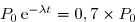
} \\\overset{ { \white{ . } } } {\phantom{P_0\,\text e^{-\lambda t}=0,7\times P_0}\quad\Longleftrightarrow\quad t=\dfrac{\ln(0,7)}{-\lambda }} \\\overset{ { \white{ . } } } {\phantom{P_0\,\text e^{-\lambda t}=0,7\times P_0}\quad\Longleftrightarrow\quad t=-\dfrac{\ln(0,7)}{1,2444\times10^{-4}}})

 Voir la correction
 forum de terminale