Pour tout entier naturel non nuln , on considère la fonction définie sur I = [0 , +[ par :
et
et soit sa courbe représentative dans un repère orthonormé
1. a) Nous devons vérifier que :
En effet,
Montrons que la fonction est continue à droite en 0.
Par définition,
Calculons
Nous en déduisons que
Par conséquent, la fonction est continue à droite en 0.
1. b) Nous devons calculer
1. c) Nous devons vérifier que :
En effet,
Calculons
Nous en déduisons que la courbe admet une branche parabolique de direction l'axe des abscisses au voisinage de +.
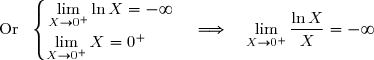
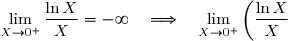
1. d) Calculons
Considérons la parité de n .
Premier cas : n est pair.
Second cas : n est impair.
Interprétation graphique du résultat.
La fonction est définie en 0 et
Dès lors,
Donc si n est pair, alors
si n est impair, alors
En conséquence, la courbe possède une demi-tangente au point de coordonnées (0 ; 0).
Cette demi-tangente est orientée vers le haut si n est pair et est orientée vers le bas si n est impair.
2. a) Montrons que est dérivable sur ]0 ; +[.
La fonction est dérivable sur ]0 ; +[ (composée de deux fonctions dérivables sur ]0 ; +[).
La fonction est dérivable sur ]0 ; +[.
D'où la fonction est dérivable sur ]0 ; +[ (produit de deux fonctions dérivables sur ]0 ; +[).
Par conséquent, est dérivable sur ]0 ; +[.
De plus,
2. b) Pour tout entier naturel
Par conséquent,
2. c) Nous devons étudier, selon la parité de n , le sens de variation de et donner son tableau de variations.
Rappelons que
Or
Donc le signe de est le signe de
Premier cas : n est pair.
Si n est pair, alors (n -1) est impair.
Dès lors, le signe de est le signe de
Calculs préliminaires :
Nous obtenons alors le tableau de variations de
Second cas : n est impair.
Supposons
Si n est impair, alors (n -1) est pair.
Dès lors,
Nous obtenons alors le tableau de variations de
Supposons
Dans ce cas,
Nous obtenons alors le tableau de variations de
2. d) Nous devons montrer que si n est impair et n 3, alors le point d'abscisse 1 est un point d'inflexion de
Les variations de lorsque n est impair et n 3 ont été étudiées dans la question 2. c) - Second cas : n est impair et différent de 1 (deuxième tableau) .
Nous observons que
Le point de coordonnées (1 ; 0) est un point stationnaire où la tangente à la courbe est horizontale.
La dérivée ne change pas de signe dans le voisinage de 1.
Par conséquent, le point stationnaire d'abscisse 1 est un point d'inflexion de
Partie II
1. Soit un réel fixé.
On considère la suite numérique définie par :
1. a) Pour tout entier naturel non nul n , nous savons par la question 2. c) - Partie I que la fonction est strictement croissante sur l'intervalle [1 ; e].
Dès lors,
1. b) Montrons que la suite est décroissante.
D'où
Par conséquent, la suite est décroissante.
1. c) Nous devons déterminer
Nous avons montré dans les questions 1. a) et 1. b) que la suite (un ) est décroissante et minorée par 0.
Selon le théorème de convergence monotone, nous en déduisons que la suite (un ) est convergente.
Nous obtenons alors,
2. a) Montrons que pour tout entier naturel n non nul, il existe un unique réel tel que :
La fonction est continue sur l'intervalle [1 ; e] (produit de deux fonctions continues sur cet intervalle).
La fonction est strictement croissante sur l'intervalle ]1 ; e[ (voir question 2. c) - Partie I).
Selon le corollaire du théorème des valeurs intermédiaires, l'équation admet une unique solution dans ]1 ; e[ .
Par conséquent, pour tout entier naturel n non nul, il existe un unique réel tel que
2. b) Nous devons montrer que la suite est croissante.
Montrons que
Dès lors, est bien défini.
Nous obtenons ainsi :
De plus, nous savons que la fonction est strictement croissante sur l'intervalle ]1 ; e[.
Nous en déduisons alors que
Par conséquent, la suite est croissante.
Nous avons montré dans les questions précédentes que la suite est croissante et majorée par e.
Selon le théorème de convergence monotone, nous en déduisons que la suite est convergente.
3. On pose :
3. a) Nous savons que
Étant donné que la suite est croissante, nous déduisons que
Mais dans un passage à la limite, une relation d'inégalité stricte devient large.
Nous obtenons alors : , soit
Or
D'où
Par conséquent,
3. b) Montrons que
Nous savons que pour tout entier naturel n non nul,
Dès lors,
D'où
Or
Par conséquent,
3. c) Montrons que si , alors
La fonction est définie et continue sur l'intervalle ]1 ; e[.
De plus,
Dès lors,
Par conséquent,
3. d) Nous devons en déduire la valeur de
Nous savons par les questions 3. a) et 3. b) que et que
Puisque la fonction est continue sur ]0 ; +[, nous en déduisons que , soit
Or nous avons montré dans la question 3. c) que si alors
Nous en déduisons que le cas est impossible sinon nous aurions , ce qui est absurde.
Par conséquent,
Partie III
On pose pour tout
1. a) Nous devons montrer que la fonction F est continue sur I .
On pose pour tout
La fonction est continue sur I car elle est continue à droite de 0 (voir Partie I - 1. a) et est continue sur ]0 ; +[ car elle est dérivable sur cet intervalle (voir Partie I - 2. a).
Nous en déduisons que la fonction est continue sur I .
Or
D'où la fonction G est dérivable sur I et par suite, la fonction G est continue sur I .
Dès lors, la fonction (-G ) est continue sur I .
Puisque F=-G , nous avons montré que la fonction F est continue sur I .
1. b) Déterminons une expression algébrique de
Calculons
Par conséquent,
2. a) Nous devons calculer
2. b) Nous devons en déduire la valeur de
Nous avons montré dans la question 1. a) que la fonction F est continue sur I .
La fonction F est donc continue à droite en 0.
Nous en déduisons que
Par conséquent,
2. c) Nous devons calculer, en cm3, le volume V du solide engendré par la rotation d'un tour complet autour de l'axe des abscisses de la portion de la courbe
relative à l'intervalle [0 ; 1]. (On prendra )
3,5 points
exercice 2
Partie I
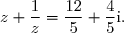
On considère dans , le système suivant :
1. Soit une solution du système (S ). On pose :
1. a) Calculons
1. b) Montrons que
Nous savons par la question 1. a) que
Dès lors,
Résolvons dans l'équation
Donc la valeur de est à exclure car
Par conséquent, l'unique solution de l'équation est
1. c) Nous devons en déduire les valeurs du couple
D'où l'unique valeur du couple est
2. Puisque , nous en déduisons que l'ensemble des solutions du système (S ) est
Partie II
Le plan est rapporté à un repère orthonormé
Soit le cercle de centre O et de rayon 1 et
trois points du cercle deux à deux distincts.
1. Montrons que
2. a) La droite passant par A et parallèle à (BC ) coupe le cercle (U ) au point P (p ).
Montrons que
D'une part, nous savons que les points appartiennent au cercle de centre O et de rayon 1.
Dès lors,
D'autre part, la droite passant par A et parallèle à (BC ) coupe le cercle (U ) au point P (p ).
Il s'ensuit que les vecteurs et sont colinéaires.
Nous obtenons alors :
2. b) La droite passant par A et perpendiculaire à (BC ) coupe le cercle (U ) au point Q (q ). Montrons que
D'une part, nous savons que le point appartient au cercle de centre O et de rayon 1.
Dès lors,
D'autre part, la droite passant par A et perpendiculaire à (BC ) coupe le cercle (U ) au point Q (q ).
Il s'ensuit que les vecteurs et sont orthogonaux.
Nous obtenons alors :
Or nous avons montré dans la question 2. a) que
Par conséquent,
2. c) La droite passant par C et parallèle à (AB ) coupe le cercle (U ) au point R (r ). Montrons que les deux droites (PR ) et (OB ) sont perpendiculaires.
En nous inspirant de la question 1. a) et en remplaçant A par C , B par A , B par B et P par R , nous obtenons :
Nous allons montrer que les vecteurs et sont orthogonaux en montrant que , soit que , soit que
Dès lors, les vecteurs et sont orthogonaux.
Nous en déduisons que les deux droites (PR ) et (OB ) sont perpendiculaires.
3,5 points
exercice 3
On rappelle que est un anneau unitaire et non commutatif d'unité
Soit
1. Nous devons montrer que E est un sous-groupe de
Nous savons que est un groupe car est un anneau.
Pour montrer que est un sous-groupe de , il suffit de montrer que la partie de comprend l'élément neutre du groupe et que
Par conséquent, est un sous-groupe de
2. On munit l'ensemble de la loi de composition interne définie par :
et on considère l'application définie de vers par :
2. a) Nous devons montrer que est un homomorphisme de vers
Nous devons également montrer que
Montrons que tout élément de possède au moins un antécédent par l'application
Soit un élément de
Nous en déduisons alors que :
D'où tout élément de possède au moins un antécédent par l'application
Par conséquent,
2. b) Montrons que est un groupe commutatif.
Nous avons montré dans la question 1 que est un sous-groupe de
Donc est un groupe commutatif car est un groupe commutatif.
Or l'image d'un groupe commutatif par un homomorphisme est un groupe commutatif.
Il s'ensuit que est un groupe commutatif.
Puisque nous déduisons que est un groupe commutatif.
3. On munit de la loi de composition interne définie par :
3. a) Nous devons montrer que la loi est commutative.
Par conséquent, la loi est commutative dans
3. b) Nous devons vérifier que (0 ; 1) est l'élément neutre de dans
D'une part,
D'autre part,
Or nous avons montré que la loi est commutative dans
Dès lors,
Nous en déduisons que
Par conséquent, (0 ; 1) est l'élément neutre de dans
3. b) Nous devons vérifier que
De plus, nous rappelons que si la loi est associative et si l'élément de possède un symétrique, alors ce symétrique est unique.
Or en utilisant la question b) et la commutativité de la loi dans nous en déduisons que :
Puisque (0 ; 1) est l'élément neutre de , il s'ensuit que l'élément (1 , i) admet une infinité de symétriques.
En vertu du rappel de la propriété ci-dessus, nous en concluons que la loi n'est pas associative dans
4. Soit
4. a) Nous devons montrer que G est un sous-groupe de .
Nous remarquons que :
La loi étant commutative dans , nous obtenons :
D'où (0 , 0) est l'élément neutre du groupe
La loi étant commutative dans , nous obtenons :
D'où est le symétrique de pour la loi
Pour montrer que G est un sous-groupe du groupe , il suffit de montrer que la partie de comprend l'élément neutre du groupe
et que
Manifestement, (0 , 0) appartient à G .
Par conséquent, G est un sous-groupe de .
4. b) Soit l'application définie de vers par :
Nous devons montrer que est un homomorphisme de vers
D'une part,
D'autre part,
D'où,
Par conséquent, est un homomorphisme de vers
4. c) Montrons que est un groupe commutatif.
Nous savons que est un groupe commutatif.
Or l'image d'un groupe commutatif par un homomorphisme est un groupe commutatif.
Il s'ensuit que est un groupe commutatif.
Nous déduisons que est un groupe commutatif.
5. Nous devons montrer que est un corps commutatif.
est un groupe commutatif car est un sous-groupe du groupe commutatif (voir question 4. a). Nous savons que est un groupe commutatif (voir question 4. c).
Montrons que est distributive par rapport à dans G .
Or la loi est commutative dans G .
Nous en déduisons que est distributive par rapport à dans G .
Par conséquent, est un corps commutatif.
3 points
exercice 4
Soit p un nombre premier impair.
On pose
Soit q un nombre premier qui divise S .
1. a) Montrons que p et q sont premiers entre eux.
Dès lors, sachant que p et q sont des entiers non nuls (car p et q sont premiers), nous déduisons qu'il existe deux entiers
u et v tels que
Il suffit de poser
Par conséquent, selon le théorème de Bézout, p et q sont premiers entre eux.
1. b) Nous savons que q est premier et que
D'après le petit théorème de Fermat, nous déduisons que
1. c)S est la somme de p termes d'une suite géométrique de raison p dont le premier terme est 1.
Nous obtenons alors :
D'où
Montrons que
Nous savons que q divise S .
Puisque (p -1) est un nombre entier, q divise
Or
Dès lors, q divise
Par conséquent,
2.On suppose quep et q -1 sont premiers entre eux.
2. a) En utilisant le théorème de Bézout, montrons que :
Nous avons supposé quep et q -1 sont premiers entre eux.
Suivant le théorème de Bézout, nous savons qu'il existe alors deux nombres entiers u et v tels que :
Montrons qu'il est impossible d'avoir (u > 0 et v 0) ou (u 0 et v 0).
Soit u > 0 et v 0.
Nous savons que u est un nombre entier et que p est un nombre premier impair.
Dès lors,
Or
Cela signifierait que : ce qui est absurde.
D'où il est impossible d'avoir (u > 0 et v 0).
Soit u 0 et v 0.
Nous obtenons alors :
Or
Cela signifierait que : ce qui est absurde.
D'où il est impossible d'avoir (u 0 et v 0).
Nous venons donc de montrer qu'il est impossible d'avoir (u > 0 et v 0) ou (u 0 et v 0).
Envisageons le cas : u > 0 et v < 0.
Nous obtenons alors :
Or selon les questions 1. b) et 1. c), nous savons que et que
En sachant que u et (-v ) sont des entiers strictement positifs, nous déduisons alors que :
Il s'ensuit que
Par conséquent,
Envisageons le cas : u 0 et v > 0.
Nous obtenons alors :
Or selon les questions 1. b) et 1. c), nous savons que et que
En sachant que (-u ) et v sont des entiers strictement positifs, nous déduisons alors que :
Il s'ensuit que
Par conséquent,
2. b) Nous devons en déduire que
3. Nous devons montrer que
Nous avons démontré dans la question 2 b) que si p et q -1 sont premiers entre eux, alors
Or q divise S , soit
Dès lors,
ce qui est impossible car k est un nombre entier et q est un nombre premier.
Par conséquent, p et q -1 ne sont pas premiers entre eux.
Or p est un nombre premier.
Donc p divise q -1, soit
Publié par malou/Panter
le
ceci n'est qu'un extrait
Pour visualiser la totalité des cours vous devez vous inscrire / connecter (GRATUIT) Inscription Gratuitese connecter
Merci à Hiphigenie / Panter pour avoir contribué à l'élaboration de cette fiche
Désolé, votre version d'Internet Explorer est plus que périmée ! Merci de le mettre à jour ou de télécharger Firefox ou Google Chrome pour utiliser le site. Votre ordinateur vous remerciera !
 définie sur I = [0 , +
 [ par :
=0 }) et
et ![\overset{ { \white{ . } } } { \forall\,x\in\,]0\;;\;+\infty[\;,\;f_n(x)=\sqrt x\,(\ln x)^n }](https://latex.ilemaths.net/latex-0.tex?\overset{ { \white{ . } } } { \forall\,x\in\,]0\;;\;+\infty[\;,\;f_n(x)=\sqrt x\,(\ln x)^n })
 }) sa courbe représentative dans un repère orthonormé
sa courbe représentative dans un repère orthonormé \,)
![\forall\,x\in\;]0\;;\;+\infty[\;,\;\sqrt x(\ln x)^n=(2n)^n\left(x^{\frac{1}{2n}}\ln\left(x^{\frac{1}{2n}}\right)\right)^n.](https://latex.ilemaths.net/latex-0.tex?\forall\,x\in\;]0\;;\;+\infty[\;,\;\sqrt x(\ln x)^n=(2n)^n\left(x^{\frac{1}{2n}}\ln\left(x^{\frac{1}{2n}}\right)\right)^n.)
![\forall\,x\in\;]0\;;\;+\infty[\;,\; (2n)^n\left(x^{\frac{1}{2n}}\ln\left(x^{\frac{1}{2n}}\right)\right)^n=(2n)^n\left(x^{\frac{1}{2n}}\times\dfrac{1}{2n}\ln x\right)^n \\\\ \phantom{WWWWWWWWWWWWWWWW}=(2n)^n\times\left(x^{\frac{1}{2n}}\right)^n\times\left(\dfrac{1}{2n}\right)^n\times(\ln x)^n \\\\ \phantom{WWWWWWWWWWWWWWWW}=(2n)^n\times x^{\frac{1}{2}}\times\dfrac{1}{(2n)^n}\times(\ln x)^n](https://latex.ilemaths.net/latex-0.tex?\forall\,x\in\;]0\;;\;+\infty[\;,\; (2n)^n\left(x^{\frac{1}{2n}}\ln\left(x^{\frac{1}{2n}}\right)\right)^n=(2n)^n\left(x^{\frac{1}{2n}}\times\dfrac{1}{2n}\ln x\right)^n \\\\ \phantom{WWWWWWWWWWWWWWWW}=(2n)^n\times\left(x^{\frac{1}{2n}}\right)^n\times\left(\dfrac{1}{2n}\right)^n\times(\ln x)^n \\\\ \phantom{WWWWWWWWWWWWWWWW}=(2n)^n\times x^{\frac{1}{2}}\times\dfrac{1}{(2n)^n}\times(\ln x)^n)
![\\\\ \phantom{WWWWWWWWWWWWWWWW}=x^{\frac{1}{2}}\times(\ln x)^n \\\\ \phantom{WWWWWWWWWWWWWWWW}=\sqrt x\times(\ln x)^n \\\\\Longrightarrow\quad\boxed{\forall\,x\in\;]0\;;\;+\infty[\;,\;\sqrt x(\ln x)^n=(2n)^n\left(x^{\frac{1}{2n}}\ln\left(x^{\frac{1}{2n}}\right)\right)^n}](https://latex.ilemaths.net/latex-0.tex?\\\\ \phantom{WWWWWWWWWWWWWWWW}=x^{\frac{1}{2}}\times(\ln x)^n \\\\ \phantom{WWWWWWWWWWWWWWWW}=\sqrt x\times(\ln x)^n \\\\\Longrightarrow\quad\boxed{\forall\,x\in\;]0\;;\;+\infty[\;,\;\sqrt x(\ln x)^n=(2n)^n\left(x^{\frac{1}{2n}}\ln\left(x^{\frac{1}{2n}}\right)\right)^n})
 Par définition,
 .})

=\lim\limits_{x\to 0^+}\sqrt x\,(\ln x)^n \\ \overset{ { \white{ . } } } { \phantom{WWWWi}=\lim\limits_{x\to 0^+}}(2n)^n\left(x^{\frac{1}{2n}}\ln\left(x^{\frac{1}{2^n}}\right)\right)^n \\ \overset{ { \white{ . } } } { \phantom{WWWWi}=(2n)^n\lim\limits_{x\to 0^+}}\left(x^{\frac{1}{2n}}\ln\left(x^{\frac{1}{2^n}}\right)\right)^n \\ \overset{ { \white{ . } } } { \phantom{WWWWi}=(2n)^n\lim\limits_{X\to 0^+}}\left(X\ln X\right)^n \quad\text{où }X=x^{\frac{1}{2n}})
^n\times0\quad\text{ (croissances comparées) }} \\ \overset{ { \white{ . } } } { \phantom{WWWWi}=0} \\\\\Longrightarrow\quad \lim\limits_{x\to 0^+}f_n(x)=0)
=f_n(0)}\,.})
. })
^n=+\infty\quad(n\in\N^*)\end{matrix}\right. \\\\\phantom{WWWWWWWW}\quad\Longrightarrow\quad\lim\limits_{x\to +\infty}\sqrt x(\ln x)^n=+\infty \\\\\phantom{WWWWWWWW}\quad\Longrightarrow\quad\boxed{\lim\limits_{x\to +\infty}f_n(x)=+\infty})
![\forall\,x\in\;]0\;;\;+\infty[\;,\;\dfrac{f_n(x)}{x}=(2n)^n\left(\dfrac{\ln\left(x^{\frac{1}{2n}}\right)}{x^{\frac{1}{2n}}}\right)^n.](https://latex.ilemaths.net/latex-0.tex?\forall\,x\in\;]0\;;\;+\infty[\;,\;\dfrac{f_n(x)}{x}=(2n)^n\left(\dfrac{\ln\left(x^{\frac{1}{2n}}\right)}{x^{\frac{1}{2n}}}\right)^n.)
![\forall\,x\in\;]0\;;\;+\infty[\;,\;\dfrac{f_n(x)}{x}=\dfrac{\sqrt x(\ln x)^n}{x} \\\\\phantom{WWWWWWWWW}=\dfrac{(2n)^n\left(x^{\frac{1}{2n}}\ln\left(x^{\frac{1}{2n}}\right)\right)^n}{x} \\\\\phantom{WWWWWWWWW}=(2n)^n\times\dfrac{\left(x^{\frac{1}{2n}}\ln\left(x^{\frac{1}{2n}}\right)\right)^n}{\left(x^{\frac{1}{n}}\right)^n} \\\\\phantom{WWWWWWWWW}=(2n)^n\times\left(\dfrac{x^{\frac{1}{2n}}\ln\left(x^{\frac{1}{2n}}\right)}{x^{\frac{1}{n}}}\right)^n](https://latex.ilemaths.net/latex-0.tex?\forall\,x\in\;]0\;;\;+\infty[\;,\;\dfrac{f_n(x)}{x}=\dfrac{\sqrt x(\ln x)^n}{x} \\\\\phantom{WWWWWWWWW}=\dfrac{(2n)^n\left(x^{\frac{1}{2n}}\ln\left(x^{\frac{1}{2n}}\right)\right)^n}{x} \\\\\phantom{WWWWWWWWW}=(2n)^n\times\dfrac{\left(x^{\frac{1}{2n}}\ln\left(x^{\frac{1}{2n}}\right)\right)^n}{\left(x^{\frac{1}{n}}\right)^n} \\\\\phantom{WWWWWWWWW}=(2n)^n\times\left(\dfrac{x^{\frac{1}{2n}}\ln\left(x^{\frac{1}{2n}}\right)}{x^{\frac{1}{n}}}\right)^n)
![\\\\\phantom{WWWWWWWWW}=(2n)^n\times\left(\dfrac{\ln\left(x^{\frac{1}{2n}}\right)}{x^{\frac{1}{n}-\frac{1}{2n}}}\right)^n \\\\\phantom{WWWWWWWWW}=(2n)^n\times\left(\dfrac{\ln\left(x^{\frac{1}{2n}}\right)}{x^{\frac{2-1}{2n}}}\right)^n \\\\\phantom{WWWWWWWWW}=(2n)^n\times\left(\dfrac{\ln\left(x^{\frac{1}{2n}}\right)}{x^{\frac{1}{2n}}}\right)^n \\\\\Longrightarrow\quad\boxed{\forall\,x\in\;]0\;;\;+\infty[\;,\;\dfrac{f_n(x)}{x}=(2n)^n\left(\dfrac{\ln\left(x^{\frac{1}{2n}}\right)}{x^{\frac{1}{2n}}}\right)^n}](https://latex.ilemaths.net/latex-0.tex?\\\\\phantom{WWWWWWWWW}=(2n)^n\times\left(\dfrac{\ln\left(x^{\frac{1}{2n}}\right)}{x^{\frac{1}{n}-\frac{1}{2n}}}\right)^n \\\\\phantom{WWWWWWWWW}=(2n)^n\times\left(\dfrac{\ln\left(x^{\frac{1}{2n}}\right)}{x^{\frac{2-1}{2n}}}\right)^n \\\\\phantom{WWWWWWWWW}=(2n)^n\times\left(\dfrac{\ln\left(x^{\frac{1}{2n}}\right)}{x^{\frac{1}{2n}}}\right)^n \\\\\Longrightarrow\quad\boxed{\forall\,x\in\;]0\;;\;+\infty[\;,\;\dfrac{f_n(x)}{x}=(2n)^n\left(\dfrac{\ln\left(x^{\frac{1}{2n}}\right)}{x^{\frac{1}{2n}}}\right)^n})
}{x}. )
}{x}=\lim\limits_{x\to +\infty}(2n)^n\left(\dfrac{\ln\left(x^{\frac{1}{2n}}\right)}{x^{\frac{1}{2n}}}\right)^n \\ \overset{ { \white{ . } } } { \phantom{WWWWix}=(2n)^n\lim\limits_{x\to +\infty}}\left(\dfrac{\ln\left(x^{\frac{1}{2n}}\right)}{x^{\frac{1}{2n}}}\right)^n \\ \overset{ { \white{ . } } } { \phantom{WWWWix}=(2n)^n\lim\limits_{X\to +\infty}}\left(\dfrac{\ln X}{X}\right)^n \quad\text{où }X=x^{\frac{1}{2n}})
^n\times0\quad\text{ (croissances comparées) }} \\ \overset{ { \white{ . } } } { \phantom{WWWWix}=0} \\\\\Longrightarrow\quad \boxed{\lim\limits_{x\to +\infty}\dfrac{f_n(x)}{x}=0})
}{x}. )
}{x}=\lim\limits_{x\to 0^+}(2n)^n\left(\dfrac{\ln\left(x^{\frac{1}{2n}}\right)}{x^{\frac{1}{2n}}}\right)^n \\ \overset{ { \white{ . } } } { \phantom{WWWWix}=(2n)^n\lim\limits_{x\to 0^+}}\left(\dfrac{\ln\left(x^{\frac{1}{2n}}\right)}{x^{\frac{1}{2n}}}\right)^n \\ \overset{ { \white{ . } } } { \phantom{WWWWix}=(2n)^n\lim\limits_{X\to 0^+}}\left(\dfrac{\ln X}{X}\right)^n \quad\text{où }X=x^{\frac{1}{2n}})
^n=+\infty\\\\\phantom{XXXXXXiXX}\quad\Longrightarrow\quad(2n)^n\lim\limits_{X\to 0^+}\left(\dfrac{\ln X}{X}\right)^n=+\infty \\\\\phantom{XXXXiXXXX}\quad\Longrightarrow\quad\boxed{\lim\limits_{x\to 0^+}\dfrac{f_n(x)}{x}=+\infty})
^n=-\infty\\\\\phantom{XXXXXXiXX}\quad\Longrightarrow\quad(2n)^n\lim\limits_{X\to 0^+}\left(\dfrac{\ln X}{X}\right)^n=-\infty \\\\\phantom{XXXXiXXXX}\quad\Longrightarrow\quad\boxed{\lim\limits_{x\to 0^+}\dfrac{f_n(x)}{x}=-\infty})
=0. })
}{x}=\lim\limits_{x\to 0^+}\dfrac{f_n(x)-0}{x-0}\quad\Longrightarrow\quad\lim\limits_{x\to 0^+}\dfrac{f_n(x)}{x}=\lim\limits_{x\to 0^+}\dfrac{f_n(x)-f_n(0)}{x-0})
 si n est pair, alors
 -f_n(0)}{x-0}=+\infty)

-f_n(0)}{x-0}=-\infty)
^n }) est dérivable sur ]0 ; +
est dérivable sur ]0 ; + est dérivable sur ]0 ; +
^n }) est dérivable sur ]0 ; +
est dérivable sur ]0 ; +![\overset{ { \white{ . } } } { \forall\,x\in\;] 0\;;\;+\infty[\,, }](https://latex.ilemaths.net/latex-0.tex?\overset{ { \white{ . } } } { \forall\,x\in\;] 0\;;\;+\infty[\,, })

![f\,'_n(x)=[\sqrt x\,(\ln x)^n ]' \\ \overset{ { \white{ . } } } { \phantom{f\,'_n(x)}=(\sqrt x)'\times(\ln x)^n+\sqrt x\times[(\ln x)^n]' } \\ \overset{ { \white{ . } } } { \phantom{f\,'_n(x)}=\dfrac{1}{2\sqrt x}\times(\ln x)^n+\sqrt x\times[n\times\dfrac{1}{x}\times(\ln x)^{n-1}] } \\ \overset{ { \white{ . } } } { \phantom{f\,'_n(x)}=\dfrac{1}{2\sqrt x}(\ln x)^n+n\times\dfrac{1}{\sqrt x}(\ln x)^{n-1} }](https://latex.ilemaths.net/latex-0.tex?f\,'_n(x)=[\sqrt x\,(\ln x)^n ]' \\ \overset{ { \white{ . } } } { \phantom{f\,'_n(x)}=(\sqrt x)'\times(\ln x)^n+\sqrt x\times[(\ln x)^n]' } \\ \overset{ { \white{ . } } } { \phantom{f\,'_n(x)}=\dfrac{1}{2\sqrt x}\times(\ln x)^n+\sqrt x\times[n\times\dfrac{1}{x}\times(\ln x)^{n-1}] } \\ \overset{ { \white{ . } } } { \phantom{f\,'_n(x)}=\dfrac{1}{2\sqrt x}(\ln x)^n+n\times\dfrac{1}{\sqrt x}(\ln x)^{n-1} })

}=\dfrac{1}{2\sqrt x}(\ln x)^{n-1}\times\ln x+2n\times\dfrac{1}{2\sqrt x}(\ln x)^{n-1} } \\ \overset{ { \white{ . } } } { \phantom{f\,'_n(x)}=\dfrac{1}{2\sqrt x}(\ln x)^{n-1}\times(\ln x+2n)})
![\\ \\ \Longrightarrow\quad\boxed{\forall\,x\in\;] 0\;;\;+\infty[\,, f\,'_n(x)=\dfrac{1}{2\sqrt x}(\ln x)^{n-1}(2n+\ln x)}](https://latex.ilemaths.net/latex-0.tex?\\ \\ \Longrightarrow\quad\boxed{\forall\,x\in\;] 0\;;\;+\infty[\,, f\,'_n(x)=\dfrac{1}{2\sqrt x}(\ln x)^{n-1}(2n+\ln x)})

=0\quad\Longleftrightarrow\quad \dfrac{1}{2\sqrt x}(\ln x)^{n-1}(2n+\ln x)=0 \\ \overset{ { \white{ . } } } { \phantom{f'_n(x)=0}\quad\Longleftrightarrow\quad (\ln x)^{n-1}(2n+\ln x)=0 \quad\text{car }\dfrac{1}{2\sqrt x}\neq0} \\ \overset{ { \white{ . } } } { \phantom{f'_n(x)=0}\quad\Longleftrightarrow\quad ((\ln x)^{n-1}=0\quad\text{ou}\quad 2n+\ln x=0) } \\ \overset{ { \white{ . } } } { \phantom{f'_n(x)=0}\quad\Longleftrightarrow\quad (\ln x=0\quad\text{ou}\quad \ln x=-2n) })

=0}\quad\Longleftrightarrow\quad (x=1\quad\text{ou}\quad x=\text e^{-2n}) })
=0\quad\Longleftrightarrow\quad (x=1\quad\text{ou}\quad x=\text e^{-2n} )})
![\overset{ { \white{ . } } } { \forall\,x\in\;] 0\;;\;+\infty[\,, f\,'_n(x)=\dfrac{1}{2\sqrt x}(\ln x)^{n-1}(2n+\ln x) }](https://latex.ilemaths.net/latex-0.tex?\overset{ { \white{ . } } } { \forall\,x\in\;] 0\;;\;+\infty[\,, f\,'_n(x)=\dfrac{1}{2\sqrt x}(\ln x)^{n-1}(2n+\ln x) })
![\overset{ { \white{ . } } } { \forall\,x\in\;] 0\;;\;+\infty[\,, \dfrac{1}{2\sqrt x}>0 }](https://latex.ilemaths.net/latex-0.tex?\overset{ { \white{ . } } } { \forall\,x\in\;] 0\;;\;+\infty[\,, \dfrac{1}{2\sqrt x}>0 })
 }) est le signe de
est le signe de ^{n-1}(2n+\ln x).)
^{n-1} ) est le signe de
est le signe de 
^{n-1}=0\Longleftrightarrow \ln x=0\\\phantom{XXxxXX}\Longleftrightarrow x=1\\ (\ln x)^{n-1}<0\Longleftrightarrow x<1\\ (\ln x)^{n-1}>0\Longleftrightarrow x>1\end{matrix}\right \\ \\ \\ \left\lbrace\begin{matrix}2n+\ln x=0\Longleftrightarrow \ln x=-2n\\ \phantom{WWWWW}\Longleftrightarrow x=\text e^{-2n}\;\\ 2n+\ln x<0\Longleftrightarrow \ln x<-2n\\ \phantom{WWWWW}\Longleftrightarrow x<\text e^{-2n}\\ 2n+\ln x>0\Longleftrightarrow x>\text e^{-2n} \end{matrix}\right. \\ \\ \\ \left\lbrace\begin{matrix}f_n(1)=\sqrt 1\times(\ln 1)^n=1\times0=0\phantom{WWWWwW}\\f_n(\text e^{-2n})=\sqrt {\text e^{-2n}}\times(\ln \text e^{-2n})^n=\text e^{-n}\times(-2n)^n\end{matrix}\right.)

^{n-1}&||&-&-&-&0&+&\\ 2n+\ln x&||& - &0& + &+ &+ & \\&||&&&&&&\\ \hline&||&&&&&& \\ f'_n(x)&||&+&0&-&0&+&\\&||&&& &&&\\ \hline&&&(-2n)^n\,\text e^{-n}&&&&+\infty\\ f_n&&\nearrow&&\searrow&&\nearrow&\\&0&&& &0&&\\ \hline \end{array})
 Supposons
^{n-1}\ge0. )
^{n-1}&||&+&+&+&0&+&\\ 2n+\ln x&||& - &0& + &+ &+ & \\&||&&&&&&\\ \hline&||&&&&&& \\ f'_n(x)&||&-&0&+&0&+&\\&||&&& &&&\\ \hline&0&&&&&&+\infty\\ f_n&&\searrow&&\nearrow&0&\nearrow&\\&&&(-2n)^n\,\text e^{-n}& &&&\\ \hline \end{array})

^{n-1}=(\ln x)^0=1. })

^{n-1}=1&||&+&+&+&\\ 2+\ln x&||& - &0& + & \\&||&&&&\\ \hline&||&&&& \\ f'_1(x)&||&-&0&+&\\&||&&& &\\ \hline&0&&&&+\infty\\ f_1&&\searrow&&\nearrow&\\&&&-2\,\text e^{-1}& &\\ \hline \end{array})
 3, alors le point d'abscisse 1 est un point d'inflexion de
 \,. })
 lorsque n est impair et n
 =0})
 }) ne change pas de signe dans le voisinage de 1.
ne change pas de signe dans le voisinage de 1.![\overset{ { \white{ . } } } { \beta\in\;]1\;;\;\text e[ }](https://latex.ilemaths.net/latex-0.tex?\overset{ { \white{ . } } } { \beta\in\;]1\;;\;\text e[ }) un réel fixé.
un réel fixé._{n\ge1}) définie par :
définie par : .)
 }) est strictement croissante sur l'intervalle [1 ; e].
est strictement croissante sur l'intervalle [1 ; e].![\beta\in\;]1\;;\;\text e[\quad\Longleftrightarrow\quad1<\beta<\text e \\ \overset{ { \white{ . } } } { \phantom{WWWW} \quad\Longrightarrow\quad f_n(1)<f_n(\beta)<f_n(\text e)} \\ \overset{ { \white{ . } } } { \phantom{WWWW} \quad\Longrightarrow\quad 0<u_n<\sqrt e\quad\text{car }\left\lbrace\begin{matrix}f_n(1)=0\phantom{WWWWWWWWWW}\\f_n(\beta)=u_n\phantom{WWWWWWWWxW}\\f_n(\text e)=\sqrt e\,(\ln\text e)^n=\sqrt e\times1^n=\sqrt \text e\end{matrix}\right.} \\\\ \Longrightarrow\quad\boxed{\forall\,n\in\N^*,\;0<u_n<\sqrt \text e}](https://latex.ilemaths.net/latex-0.tex?\beta\in\;]1\;;\;\text e[\quad\Longleftrightarrow\quad1<\beta<\text e \\ \overset{ { \white{ . } } } { \phantom{WWWW} \quad\Longrightarrow\quad f_n(1)<f_n(\beta)<f_n(\text e)} \\ \overset{ { \white{ . } } } { \phantom{WWWW} \quad\Longrightarrow\quad 0<u_n<\sqrt e\quad\text{car }\left\lbrace\begin{matrix}f_n(1)=0\phantom{WWWWWWWWWW}\\f_n(\beta)=u_n\phantom{WWWWWWWWxW}\\f_n(\text e)=\sqrt e\,(\ln\text e)^n=\sqrt e\times1^n=\sqrt \text e\end{matrix}\right.} \\\\ \Longrightarrow\quad\boxed{\forall\,n\in\N^*,\;0<u_n<\sqrt \text e})
-f_n(\beta) \\ \overset{ { \white{ . } } } { \phantom{\forall\,n\in\N^*,\;u_{n+1}-u_n}=\sqrt \beta\,(\ln \beta)^{n+1}-\sqrt \beta\,(\ln \beta)^{n} } \\ \overset{ { \white{ . } } } { \phantom{\forall\,n\in\N^*,\;u_{n+1}-u_n}=\sqrt \beta\,(\ln \beta)^{n}(\ln \beta-1) })
^n>0\\\ln\beta-1<0\end{matrix}\right. \\\\\phantom{WWWWiW}\quad\Longrightarrow\quad \sqrt \beta\,(\ln \beta)^{n}(\ln \beta-1)<0)

^n=0 } \\ \overset{ { \white{ . } } } { \phantom{1<\beta<\text e}\quad\Longrightarrow\quad\lim\limits_{n\to+\infty}\sqrt\beta\,(\ln \beta)^n=\sqrt\beta\times0=0 } \\ \overset{ { \phantom{ . } } } { \phantom{1<\beta<\text e}\quad\Longrightarrow\quad\boxed{\lim\limits_{n\to+\infty}u_n=0} })
![\overset{ { \white{ . } } } { x_n\in\;]1\;;\;\text e[ }](https://latex.ilemaths.net/latex-0.tex?\overset{ { \white{ . } } } { x_n\in\;]1\;;\;\text e[ }) tel que :
tel que : =1. })
 est continue sur l'intervalle [1 ; e] (produit de deux fonctions continues sur cet intervalle).
![\left\lbrace\begin{matrix}f_n(1)=0{\;\red{<1}}\phantom{ WWWWWWWWWw }\\f_n(\text e)=\sqrt e(\ln \text e)^n=\sqrt e\times1=\sqrt e{\;\red{>1}} \end{matrix}\right.\quad\Longrightarrow\quad \boxed{1\in\,]\,f_n(1)\;;\;f_n(\text e)\,[ }](https://latex.ilemaths.net/latex-0.tex?\left\lbrace\begin{matrix}f_n(1)=0{\;\red{<1}}\phantom{ WWWWWWWWWw }\\f_n(\text e)=\sqrt e(\ln \text e)^n=\sqrt e\times1=\sqrt e{\;\red{>1}} \end{matrix}\right.\quad\Longrightarrow\quad \boxed{1\in\,]\,f_n(1)\;;\;f_n(\text e)\,[ })
=1 } }) admet une unique solution
admet une unique solution  dans ]1 ; e[ .
![\overset{ { \white{ . } } } { x_n\in\; ]\,1\;;\;\text e\,[ }](https://latex.ilemaths.net/latex-0.tex?\overset{ { \white{ . } } } { x_n\in\; ]\,1\;;\;\text e\,[ }) tel que
tel que =1\,.})
_{n\in\N^*}) est croissante.
est croissante.
![\overset{ { \white{ . } } } { x_n\in\; ]\,1\;;\;\text e\,[\quad\Longrightarrow\quad x_n>0. }](https://latex.ilemaths.net/latex-0.tex?\overset{ { \white{ . } } } { x_n\in\; ]\,1\;;\;\text e\,[\quad\Longrightarrow\quad x_n>0. })
}) est bien défini.
est bien défini.

=\sqrt{x_n}\,(\ln x_n)^{n+1} \\ \overset{ { \white{ . } } } { \phantom{f_{n+1}(x_n)}=\sqrt{x_n}\,(\ln x_n)^{n}\times \ln x_n} \\ \overset{ { \white{ . } } } { \phantom{f_{n+1}(x_n)}=f_n(x_n)\times \ln x_n} \\ \overset{ { \white{ . } } } { \phantom{f_{n+1}(x_n)}=1\times \ln x_n}\quad\text{(voir question 2. a)})
}=\ln x_n} \\ \\ \Longrightarrow f_{n+1}(x_n)=\ln x_n)
![\\ \\ \text{Or }\;x_n\in\;]\,1\;;\;\text e\,[\quad\Longrightarrow\quad x_n<\text e \\ \overset{ { \white{ . } } } { \phantom{WWWWWW}\quad\Longrightarrow\quad \ln x_n<\ln \text e } \\ \overset{ { \white{ . } } } { \phantom{WWWWWW}\quad\Longrightarrow\quad \ln x_n<1 } \\ \overset{ { \white{ . } } } { \phantom{WWWWWW}\quad\Longrightarrow\quad \ln x_n<f_{n+1}(x_{n+1}) }](https://latex.ilemaths.net/latex-0.tex?\\ \\ \text{Or }\;x_n\in\;]\,1\;;\;\text e\,[\quad\Longrightarrow\quad x_n<\text e \\ \overset{ { \white{ . } } } { \phantom{WWWWWW}\quad\Longrightarrow\quad \ln x_n<\ln \text e } \\ \overset{ { \white{ . } } } { \phantom{WWWWWW}\quad\Longrightarrow\quad \ln x_n<1 } \\ \overset{ { \white{ . } } } { \phantom{WWWWWW}\quad\Longrightarrow\quad \ln x_n<f_{n+1}(x_{n+1}) })
=\ln x_n\\\overset{ { \white{ . } } } { \ln x_n<f_{n+1}(x_{n+1}) }\end{matrix}\right.\quad\Longrightarrow\quad \boxed{f_{n+1}(x_n)<f_{n+1}(x_{n+1})})
 est strictement croissante sur l'intervalle ]1 ; e[.
![\overset{ { \white{ . } } } { \forall\,n\in\N^*,\quad x_n\in\,]1\;;\;\text e\,[\quad\Longrightarrow\quad x_n<\text e.}](https://latex.ilemaths.net/latex-0.tex?\overset{ { \white{ . } } } { \forall\,n\in\N^*,\quad x_n\in\,]1\;;\;\text e\,[\quad\Longrightarrow\quad x_n<\text e.})
_{n\in\N^*}}) est croissante, nous déduisons que
est croissante, nous déduisons que 
 , soit
![\overset{ { \white{ . } } } { x_1\in\,]1\;;\;\text e\,[\quad\Longrightarrow\quad 1<x_1.}](https://latex.ilemaths.net/latex-0.tex?\overset{ { \white{ . } } } { x_1\in\,]1\;;\;\text e\,[\quad\Longrightarrow\quad 1<x_1.})

^n=\dfrac{1}{\sqrt \ell}\,.})
![\left\lbrace\begin{matrix}x_n\in\; ]\,1\;;\;\text e\,[\\\overset{ { \white{ . } } } { f_n(x_n)=1 }\end{matrix}\right. \quad\Longrightarrow\quad \left\lbrace\begin{matrix}x_n\neq 0\\\overset{ { \white{ . } } } {\sqrt x_n\,(\ln x_n)^n =1}\end{matrix}\right. \\ \\ \phantom{WWWiWW}\quad\Longrightarrow\quad \left\lbrace\begin{matrix}x_n\neq 0\\\overset{ { \white{ . } } } {(\ln x_n)^n =\dfrac{1}{\sqrt x_n}}\end{matrix}\right.](https://latex.ilemaths.net/latex-0.tex?\left\lbrace\begin{matrix}x_n\in\; ]\,1\;;\;\text e\,[\\\overset{ { \white{ . } } } { f_n(x_n)=1 }\end{matrix}\right. \quad\Longrightarrow\quad \left\lbrace\begin{matrix}x_n\neq 0\\\overset{ { \white{ . } } } {\sqrt x_n\,(\ln x_n)^n =1}\end{matrix}\right. \\ \\ \phantom{WWWiWW}\quad\Longrightarrow\quad \left\lbrace\begin{matrix}x_n\neq 0\\\overset{ { \white{ . } } } {(\ln x_n)^n =\dfrac{1}{\sqrt x_n}}\end{matrix}\right. )
^n =\lim\limits_{n\to+\infty}\dfrac{1}{\sqrt x_n}})

^n =\dfrac{1}{\sqrt \ell}}})
 , alors
  =-\infty\,.})
}) est définie et continue sur l'intervalle ]1 ; e[.
est définie et continue sur l'intervalle ]1 ; e[.![\overset{ { \white{ . } } } { \lim\limits_{n\to+\infty} x_n=\ell\in\;]1\;;\;\text e\,[\,.}](https://latex.ilemaths.net/latex-0.tex?\overset{ { \white{ . } } } { \lim\limits_{n\to+\infty} x_n=\ell\in\;]1\;;\;\text e\,[\,.})
) =\ln(\ln\ell)\,.})
<\ln1 } \\ \overset{ { \white{ . } } } {\phantom{\text{Or }\;\ell<\text e}\quad\Longrightarrow\quad \ln(\ln\ell)<0 })
<0 \\\lim\limits_{n\to+\infty}n=+\infty\end{matrix}\right.\quad\Longrightarrow\quad\boxed{\lim\limits_{n\to+\infty} n\ln( \ln x_n) =-\infty})

 et que
 ^n =\dfrac{1}{\sqrt \ell}})
 est continue sur ]0 ; +
^n =\ln\left(\dfrac{1}{\sqrt \ell}\right)}) , soit
, soit  =\ln\left(\dfrac{1}{\sqrt \ell}\right)}\,.})
 alors
alors  =-\infty. })
 est impossible sinon nous aurions
 =-\infty}) , ce qui est absurde.
, ce qui est absurde.
=\displaystyle\int_x^{1}(f_1(t))^2\text{ d}t. })
=\displaystyle\int_1^{x}(f_1(t))^2\text{ d}t. })
 est continue sur I car elle est continue à droite de 0 (voir Partie I - 1. a) et est continue sur ]0 ; +
)^2) est continue sur I .
est continue sur I .
. })
=\displaystyle\int_x^{1}(f_1(t))^2\text{ d}t \\\overset{}{\phantom{F(x)}}=\displaystyle\int_x^{1}(\sqrt t\,\ln t)^2\text{ d}t \\\overset{}{\phantom{F(x)}}=\displaystyle\int_x^{1}t\,\ln^2 t\text{ d}t)
![\underline{\text{Formule de l'intégrale par parties}}\ :\ {\blue{\displaystyle\int_x^{1}u(t)v'(t)\,\text{d}t=\left[\overset{}{u(t)v(t)}\right]\limits_x^1- \displaystyle\int\limits_x^1u'(t)v(t)\,\text{d}t}}. \\ \\ \left\lbrace\begin{matrix}u(t)=\ln^2 t\quad\Longrightarrow\quad u'(t)=2\times\dfrac{1}{t}\times\ln t \\v'(t)=t\quad\quad\quad\Longrightarrow\quad v(t)=\dfrac{t^2}{2}\phantom{WWW}\end{matrix}\right. \\ \\ \text{Dès lors, }\ F(x)= \left[\overset{}{\dfrac{t^2}{2}\ln^2 t}\right]\limits_x^1-\displaystyle\int\limits_x^12\times\dfrac{1}{t}\times\ln t\times\dfrac{t^2}{2}\,\text{d}t \\ \\ \phantom{WWWWWW}=\left[\overset{}{\dfrac{t^2}{2}\ln^2 t}\right]\limits_x^1-\displaystyle\int\limits_x^1t\times\ln t\,\text{d}t](https://latex.ilemaths.net/latex-0.tex?\underline{\text{Formule de l'intégrale par parties}}\ :\ {\blue{\displaystyle\int_x^{1}u(t)v'(t)\,\text{d}t=\left[\overset{}{u(t)v(t)}\right]\limits_x^1- \displaystyle\int\limits_x^1u'(t)v(t)\,\text{d}t}}. \\ \\ \left\lbrace\begin{matrix}u(t)=\ln^2 t\quad\Longrightarrow\quad u'(t)=2\times\dfrac{1}{t}\times\ln t \\v'(t)=t\quad\quad\quad\Longrightarrow\quad v(t)=\dfrac{t^2}{2}\phantom{WWW}\end{matrix}\right. \\ \\ \text{Dès lors, }\ F(x)= \left[\overset{}{\dfrac{t^2}{2}\ln^2 t}\right]\limits_x^1-\displaystyle\int\limits_x^12\times\dfrac{1}{t}\times\ln t\times\dfrac{t^2}{2}\,\text{d}t \\ \\ \phantom{WWWWWW}=\left[\overset{}{\dfrac{t^2}{2}\ln^2 t}\right]\limits_x^1-\displaystyle\int\limits_x^1t\times\ln t\,\text{d}t )

![\underline{\text{Formule de l'intégrale par parties}}\ :\ {\blue{\displaystyle\int_x^{1}w(t)v'(t)\,\text{d}t=\left[\overset{}{w(t)v(t)}\right]_x^1-\displaystyle\int\limits_x^1w'(t)v(t)\,\text{d}t}}. \\ \\ \left\lbrace\begin{matrix}w(t)=\ln t\quad\Longrightarrow\quad w'(t)=\dfrac{1}{t}\\\\v'(t)=t\quad\quad\Longrightarrow\quad v(t)=\dfrac{t^2}{2}\end{matrix}\right. \\ \\ \text{Dès lors, }\ \displaystyle\int\limits_x^1t\times\ln t\,\text{d}t=\left[\overset{}{\dfrac{t^2}{2}\ln t}\right]\limits_x^1-\displaystyle\int\limits_x^1\dfrac{1}{t}\times\dfrac{t^2}{2}\,\text{d}t \\ \\ \phantom{WWWWWWWWw}=\left[\overset{}{\dfrac{t^2}{2}\ln t}\right]\limits_x^1-\dfrac{1}{2}\displaystyle\int\limits_x^1t\,\text{d}t](https://latex.ilemaths.net/latex-0.tex?\underline{\text{Formule de l'intégrale par parties}}\ :\ {\blue{\displaystyle\int_x^{1}w(t)v'(t)\,\text{d}t=\left[\overset{}{w(t)v(t)}\right]_x^1-\displaystyle\int\limits_x^1w'(t)v(t)\,\text{d}t}}. \\ \\ \left\lbrace\begin{matrix}w(t)=\ln t\quad\Longrightarrow\quad w'(t)=\dfrac{1}{t}\\\\v'(t)=t\quad\quad\Longrightarrow\quad v(t)=\dfrac{t^2}{2}\end{matrix}\right. \\ \\ \text{Dès lors, }\ \displaystyle\int\limits_x^1t\times\ln t\,\text{d}t=\left[\overset{}{\dfrac{t^2}{2}\ln t}\right]\limits_x^1-\displaystyle\int\limits_x^1\dfrac{1}{t}\times\dfrac{t^2}{2}\,\text{d}t \\ \\ \phantom{WWWWWWWWw}=\left[\overset{}{\dfrac{t^2}{2}\ln t}\right]\limits_x^1-\dfrac{1}{2}\displaystyle\int\limits_x^1t\,\text{d}t )

![\\ \\ \phantom{WWWWWWWWw}=\left[\overset{}{\dfrac{t^2}{2}\ln t}\right]_x^1-\dfrac{1}{2}\left[\dfrac{t^2}{2}\right]_x^1 \\ \\ \phantom{WWWWWWWWw}=\left[\overset{}{\dfrac{t^2}{2}\ln t}\right]\limits_x^1-\dfrac{1}{4}\left[\overset{}{t^2}\right]_x^1](https://latex.ilemaths.net/latex-0.tex?\\ \\ \phantom{WWWWWWWWw}=\left[\overset{}{\dfrac{t^2}{2}\ln t}\right]_x^1-\dfrac{1}{2}\left[\dfrac{t^2}{2}\right]_x^1 \\ \\ \phantom{WWWWWWWWw}=\left[\overset{}{\dfrac{t^2}{2}\ln t}\right]\limits_x^1-\dfrac{1}{4}\left[\overset{}{t^2}\right]_x^1)
![F(x)=\left[\overset{}{\dfrac{t^2}{2}\,\ln^2 t}\right]_x^1-\left(\left[\overset{}{\dfrac{t^2}{2}\ln t}\right]_x^1-\dfrac{1}{4}\left[\overset{}{t^2}\right]_x^1\right) \\ \overset{ { \white{ . } } } { \phantom{F(x)}=\left[\overset{}{\dfrac{t^2}{2}\,\ln^2 t}\right]_x^1-\left[\overset{}{\dfrac{t^2}{2}\ln t}\right]_x^1+\dfrac{1}{4}\left[\overset{}{t^2}\right]_x^1} \\ \overset{ { \white{ . } } } { \phantom{F(x)}=\left[\overset{}{\dfrac{1^2}{2}\,\ln^2 1-\dfrac{x^2}{2}\,\ln^2 x}\right]-\left[\overset{}{\dfrac{1^2}{2}\ln 1-\dfrac{x^2}{2}\ln x}\right]+\dfrac{1}{4}(1^2-x^2)} \\ \overset{ { \white{ . } } } { \phantom{F(x)}=\left[\overset{}{0-\dfrac{x^2}{2}\,\ln^2 x}\right]-\left[\overset{}{0-\dfrac{x^2}{2}\ln x}\right]+\dfrac{1}{4}(1-x^2)} \\ \\ \\ \Longrightarrow\quad\boxed{F(x)=-\dfrac{x^2}{2}\,\ln^2 x+\dfrac{x^2}{2}\ln x+\dfrac{1}{4}(1-x^2)}](https://latex.ilemaths.net/latex-0.tex?F(x)=\left[\overset{}{\dfrac{t^2}{2}\,\ln^2 t}\right]_x^1-\left(\left[\overset{}{\dfrac{t^2}{2}\ln t}\right]_x^1-\dfrac{1}{4}\left[\overset{}{t^2}\right]_x^1\right) \\ \overset{ { \white{ . } } } { \phantom{F(x)}=\left[\overset{}{\dfrac{t^2}{2}\,\ln^2 t}\right]_x^1-\left[\overset{}{\dfrac{t^2}{2}\ln t}\right]_x^1+\dfrac{1}{4}\left[\overset{}{t^2}\right]_x^1} \\ \overset{ { \white{ . } } } { \phantom{F(x)}=\left[\overset{}{\dfrac{1^2}{2}\,\ln^2 1-\dfrac{x^2}{2}\,\ln^2 x}\right]-\left[\overset{}{\dfrac{1^2}{2}\ln 1-\dfrac{x^2}{2}\ln x}\right]+\dfrac{1}{4}(1^2-x^2)} \\ \overset{ { \white{ . } } } { \phantom{F(x)}=\left[\overset{}{0-\dfrac{x^2}{2}\,\ln^2 x}\right]-\left[\overset{}{0-\dfrac{x^2}{2}\ln x}\right]+\dfrac{1}{4}(1-x^2)} \\ \\ \\ \Longrightarrow\quad\boxed{F(x)=-\dfrac{x^2}{2}\,\ln^2 x+\dfrac{x^2}{2}\ln x+\dfrac{1}{4}(1-x^2)})
. } )
= \underset {x>0}{\lim\limits_{x\to0}}\,\left(-\dfrac{x^2}{2}\,\ln^2 x+\dfrac{x^2}{2}\ln x+\dfrac{1}{4}(1-x^2)\right) \\\\\phantom{ \underset {x>0}{\lim\limits_{x\to0}}\,F(x)}= -\dfrac{1}{2\,}\underset {x>0}{\lim\limits_{x\to0}}\,x^2\,\ln^2 x+\dfrac{1}{2\,}\underset {x>0}{\lim\limits_{x\to0}}\,x^2\,\ln x+\dfrac{1}{4}\underset {x>0}{\lim\limits_{x\to0}}\,(1-x^2)\right))
^2=0\quad\text{(croissances comparées)}\\\overset{ { \white{ . } } } { \underset {x>0}{\lim\limits_{x\to0}}\,x^2\,\ln x=0\quad\text{(croissances comparées)}}\phantom{WWWWWWW}\\\overset{ { \phantom{ . } } } { \underset {x>0}{\lim\limits_{x\to0}}(1-x^2)=1}\phantom{WWWWWWWWWWWWWWWWW}\end{matrix}\right)
=-\dfrac{1}{2}\times0+\dfrac{1}{2}\times0+\dfrac{1}{4}\times1\quad\Longrightarrow\quad\boxed{\underset {x>0}{\lim\limits_{x\to0}}\,F(x)=\dfrac{1}{4}})
. } )
=F(0). })
=\dfrac{1}{4}}\,.)
 }) relative à l'intervalle [0 ; 1]. (On prendra
relative à l'intervalle [0 ; 1]. (On prendra  )
))^2\text{d} t \\ \overset{ { \white{ . } } } { \phantom{V}=\pi\times F(0)\quad(\text{par définition de }F(x))} \\ \overset{ { \white{ . } } } { \phantom{V}=\pi\times\dfrac{1}{4}\quad(\text{voir exercice 2.}b)} \\\\\Longrightarrow\boxed{V=\dfrac{\pi}{4}\,\text{cm}^3})
 , le système suivant :
 :\left\lbrace\begin{matrix}\sqrt x\left(1+\dfrac{1}{x+y}\right)=\dfrac{12}{5}\\\overset{ { \white{ . } } } { \sqrt y\left(1-\dfrac{1}{x+y}\right)=\dfrac{4}{5}}\end{matrix}\right.)
\in\R_+^2}) une solution du système (S ). On pose :
une solution du système (S ). On pose : 

(\sqrt x-\text i\sqrt y)}} \\ \overset{ { \white{ . } } } { \phantom{z+\dfrac{1}{z}}=\sqrt x+\text i\sqrt y+\dfrac{\sqrt x-\text i\sqrt y}{x +y}} \\ \overset{ { \white{ . } } } { \phantom{z+\dfrac{1}{z}}=\sqrt x+\text i\sqrt y+\dfrac{\sqrt x}{x +y}-\text i\dfrac{\sqrt y}{x+y}})
+\left(\text i\sqrt y-\dfrac{\text i\sqrt y}{x+y}\right)} \\ \overset{ { \white{ . } } } { \phantom{z+\dfrac{1}{z}}=\sqrt x\left(1+\dfrac{1}{x +y}\right)+\text i\sqrt y\left(1-\dfrac{1}{x+y}\right)} \\ \overset{ { \white{ . } } } { \phantom{z+\dfrac{1}{z}}=\dfrac{12}{5}+\dfrac 4 5\text i} \\\\\Longrightarrow\quad\boxed{z+\dfrac{1}{z}=\dfrac{12}{5}+\dfrac 4 5\text i})
 Montrons que
 z+1=0.})
z} \\ \overset{ { \white{ . } } } { \phantom{WWWwWWW}\quad\Longleftrightarrow\quad \boxed{z^2-\left(\dfrac{12}{5}+\dfrac 4 5\text i\right)z+1=0}})
 l'équation
 ![\underline{\text{Discriminant}}:\Delta=\left[-\left(\dfrac{12}{5}+\dfrac 4 5\text i\right)\right]^2-4\times1\times1=\left(\dfrac{12}{5}+\dfrac 4 5\text i\right)^2-4 \\\overset{ { \white{ . } } } { \phantom{WWWWwWW}=\left(\dfrac{144}{25}+\dfrac {96}{25}\text i-\dfrac {16}{25}\right)-4 } \\\overset{ { \white{ . } } } { \phantom{WWWWwWW}=\dfrac{28}{25}+\dfrac {96}{25}\text i }](https://latex.ilemaths.net/latex-0.tex?\underline{\text{Discriminant}}:\Delta=\left[-\left(\dfrac{12}{5}+\dfrac 4 5\text i\right)\right]^2-4\times1\times1=\left(\dfrac{12}{5}+\dfrac 4 5\text i\right)^2-4 \\\overset{ { \white{ . } } } { \phantom{WWWWwWW}=\left(\dfrac{144}{25}+\dfrac {96}{25}\text i-\dfrac {16}{25}\right)-4 } \\\overset{ { \white{ . } } } { \phantom{WWWWwWW}=\dfrac{28}{25}+\dfrac {96}{25}\text i })

 } \\\overset{ { \phantom{ . } } } { \phantom{WWWWwWW}=\left(\dfrac{2}{5}\right)^2(4+3\,\text i)^2\quad\text{car } (4+3\,\text i)^2=16+24\text i-9=7+24\text i} \\\overset{ { \phantom{ . } } } { \phantom{WWWWwWW}=\left(\dfrac{2}{5}(4+3\,\text i)\right)^2})
}{2}=\dfrac{\dfrac{12}{5}+\dfrac 4 5\text i+\dfrac{8}{5}+\dfrac 6 5\,\text i}{2}=2+\text i \\\overset{ { \white{ . } } } { z_2=\dfrac{\dfrac{12}{5}+\dfrac 4 5\text i-\dfrac{2}{5}(4+3\,\text i)}{2}=\dfrac{\dfrac{12}{5}+\dfrac 4 5\text i-\dfrac{8}{5}-\dfrac 6 5\,\text i}{2}=\dfrac 2 5-\dfrac 1 5\text i } \\\\\text{Or }\overset{ { \white{ . } } } {z=\sqrt x+\text i\sqrt y } \quad\Longrightarrow\quad\text{Im}(z)\ge0)
 est à exclure car
 <0.})
z+1=0}) est
est 
\,.})
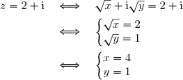
}) est
est =(4,1)}\,.})
\in\R^2_+ } ) , nous en déduisons que l'ensemble des solutions du système (S ) est
, nous en déduisons que l'ensemble des solutions du système (S ) est
 \rbrace .})
.})
 } ) le cercle de centre O et de rayon 1 et
le cercle de centre O et de rayon 1 et
,\;B(b),\;C(c) } ) trois points du cercle
trois points du cercle \quad ;\quad|z|=1\quad\Longleftrightarrow\quad \overline{z}=\dfrac 1 z. } )
\quad ;\quad|z|=1\quad\Longleftrightarrow\quad |z|^2=1 \\ \overset{ { \white{ . } } } { \phantom{WWWwWWWWW}\quad\Longleftrightarrow\quad z\overline{z}=1 } \\ \overset{ { \white{ . } } } { \phantom{WWWwWWWWW}\quad\Longleftrightarrow\quad \overline{z}=\dfrac{1}{z} } \\\\\Longrightarrow\quad\boxed{(\forall\,z\in\C)\quad ;\quad|z|=1\quad\Longleftrightarrow\quad\overline{z}=\dfrac{1}{z} })
 Montrons que
,\;B(b),\;C(c),P(p) } ) appartiennent au cercle
appartiennent au cercle 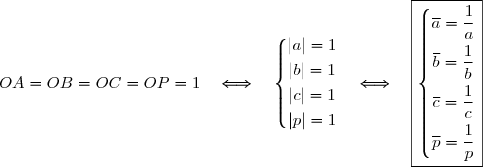
 et
et  sont colinéaires.
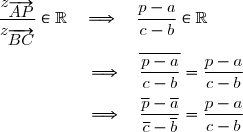
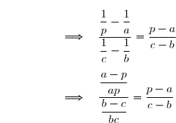

}{ap(b-c)}=\dfrac{a-p}{b-c}} \\ \overset{ { \white{ ^. } } } { \phantom{WWWW}\quad\Longrightarrow\quad\dfrac{bc}{ap}=1} \\ \overset{ { \phantom{ ^. } } } { \phantom{WWWW}\quad\Longrightarrow\quad bc=ap} \\ \overset{ { \phantom{ ^. } } } { \phantom{WWWW}\quad\Longrightarrow\quad \boxed{p=\dfrac{bc}{a}}} )

 } ) appartient au cercle
appartient au cercle 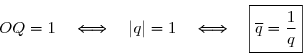
 et
et 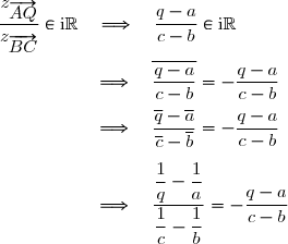
}{aq(b-c)}=-\dfrac{a-q}{b-c}} \\ \overset{ { \white{ ^. } } } { \phantom{WWWW}\quad\Longrightarrow\quad\dfrac{bc}{aq}=-1} \\ \overset{ { \phantom{ ^. } } } { \phantom{WWWW}\quad\Longrightarrow\quad bc=-aq} \\ \overset{ { \phantom{ ^. } } } { \phantom{WWWW}\quad\Longrightarrow\quad q=-\dfrac{bc}{a}} )


 et
et  sont orthogonaux en montrant que
  , soit que
  , soit que
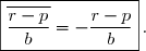
}{b}} \\\\ \phantom{WWWW}=\overline{\dfrac{a}{c}-\dfrac{c}{a}}=\dfrac{\overline a}{\overline c}-\dfrac{\overline c}{\overline a} \\\\\phantom{WWWW}=\dfrac{\dfrac 1 a}{\dfrac 1 c}-\dfrac{\dfrac 1 c}{\dfrac 1 a}=\dfrac 1 a\times\dfrac c 1-\dfrac 1 c\times\dfrac a 1 \\\\ \phantom{WWWW}=\dfrac c a-\dfrac a c=-\left(\dfrac a c-\dfrac c a\right))
}{b} \\\\ \phantom{WWWW}=\dfrac{a}{c}-\dfrac{c}{a} \\\\\text{D'où }\;\boxed{\overline{\dfrac{r-p}{b}}=-\dfrac{r-p}{b}})
,+,\times )} ) est un anneau unitaire et non commutatif d'unité
est un anneau unitaire et non commutatif d'unité 
=\begin{pmatrix}a&0&0\\0&b&-c\\0&c&b\end{pmatrix} /\;(a,b,c)\in\R^3 \right\rbrace}\,.)
,+ ) \,. } )
,+)}) est un groupe car
est un groupe car ,+,\times)}) est un anneau.
est un anneau. est un sous-groupe de
 }) comprend l'élément neutre du groupe
comprend l'élément neutre du groupe 
=\begin{pmatrix}a&0&0\\0&b&-c\\0&c&b\end{pmatrix} \in E\quad\text{avec } a=b=c=0. \\\overset{ { \white{ . } } } { \phantom{xxx} M(0,0,0)=\begin{pmatrix}0&0&0\\0&0&-0\\0&0&0\end{pmatrix}\in E }\quad\Longrightarrow\quad M(0,0,0)=\begin{pmatrix}0&0&0\\0&0&0\\0&0&0\end{pmatrix}\in E \\\phantom{WWWWWWWWWWWwW}\phantom{xxx}\quad\Longrightarrow\quad \boxed{O\in E})
\in E\text{ et }M'(a',b',c')\in E \\\overset{ { \white{ . } } } { \phantom{xxi} \text{Alors }\;M(a,b,c)-M'(a',b',c') }=\begin{pmatrix}a&0&0\\0&b&-c\\0&c&b\end{pmatrix} -\begin{pmatrix}a'&0&0\\0&b'&-c'\\0&c'&b'\end{pmatrix} \\ \overset{ { \white{ . } } } { \phantom{WWWWWWWWWWWWWw} =\begin{pmatrix}a-a'&0&0\\0&b-b'&-c+c'\\0&c-c'&b-b'\end{pmatrix} } \\ \overset{ { \phantom{ . } } } { \phantom{WWWWWWWWWWWWWw} =\begin{pmatrix}a-a'&0&0\\0&b-b'&-(c-c')\\0&c-c'&b-b'\end{pmatrix} } \\ \overset{ { \white{ . } } } { \phantom{WWWWWWWWWWWWWw}=M(a-a',b-b',c-c') \in E } \\\\\Longrightarrow\quad\boxed{\forall\,M(a,b,c)\in E,M'(a',b',c')\in E : M(a,b,c)-M'(a',b',c')\in E})
,+)\,.})
 de la loi de composition interne
  définie par :
,(x,z'))\in(\R\times \C)^2:(x,z)*(x',z')=(x+x',z+z'))
 définie de
  vers
vers  par :
par : \in\R^3, \varphi(M(a,b,c))=(a,b+c\,\text i))
) vers
vers \,.)
,M'(a',b',c'))\in E^2, \\\\\phantom{xxxx}\varphi(M(a,b,c)+M'(a',b',c'))=\varphi(M(a+a',b+b',c+c')) \\\overset{ { \white{ . } } } { \phantom{xxxx\varphi(M(a,b,c)+M'(a',b',c'))}=(a+a',b+b'+(c+c')\,\text i)} \\\overset{ { \white{ . } } } { \phantom{xxxx\varphi(M(a,b,c)+M'(a',b',c'))}=(a+a',b+b'+c\,\text i+c'\,\text i)} \\\overset{ { \white{ . } } } { \phantom{xxxx\varphi(M(a,b,c)+M'(a',b',c'))}=(a+a',b+c\,\text i+b'+c'\,\text i)})
+M'(a',b',c'))}=(a,b+c\,\text i)*(a',b'+c'\,\text i)} \\\overset{ { \white{ . } } } { \phantom{xxxx\varphi(M(a,b,c)+M'(a',b',c'))}=\varphi(M(a,b,c))*\varphi(M'(a',b',c'))} \\\\\Longrightarrow\quad\boxed{\forall\; (M(a,b,c),M'(a',b',c'))\in E^2,\varphi(M(a,b,c)+M'(a',b',c'))=\varphi(M(a,b,c))*\varphi(M'(a',b',c'))})
=\R\times\C \,. } )
 possède au moins un antécédent par l'application
 } ) un élément de
un élément de 
\in\R^2:\left\lbrace\begin{matrix}a\in\R\phantom{xxx}\\z=x+\text i\,y\end{matrix}\right. \\\overset{ { \white{ . } } } { \phantom{WWW}\quad\Longrightarrow\quad\exists\,(x,y)\in\R^2:(a,z)=(a,x+\text i\,y)} \\\overset{ { \white{ . } } } { \phantom{WWW}\quad\Longrightarrow\quad\exists\,(x,y)\in\R^2:(a,z)=\varphi(M(a,x,y))})
\in\R\times \C,\;\exists\,M(a,x,y)\in E:\varphi(M(a,x,y))=(a,z).)
=\R\times\C }\,. } )
 }) est un groupe commutatif.
est un groupe commutatif. est un sous-groupe de
 ,+) })
,*) }) est un groupe commutatif.
est un groupe commutatif.=\R\times\C\,, }) nous déduisons que
nous déduisons que  définie par :
 ,(x',z')\in(\R\times \C)^2,\;(x,z)\top (x',z')=(x\,\text{Re}(z')+x'\,\text{Re}(z),zz'))
,(x',z')\in(\R\times \C)^2,\;(x,z)\top (x',z')=(x\,\text{Re}(z')+x'\,\text{Re}(z),zz') \\ \overset{ { \white{ . } } } { \phantom{\forall\,((x,z),(x',z')\in(\R\times \C)^2,\;(x,z)\top (x',z')}= (x'\,\text{Re}(z)+x\,\text{Re}(z'),z'z) } \\ \overset{ { \white{ . } } } { \phantom{\forall\,((x,z),(x',z')\in(\R\times \C)^2,\;(x,z)\top (x',z')}=(x',z')\top (x,z)} \\\\\Longrightarrow\boxed{\forall\,((x,z),(x',z')\in(\R\times \C)^2,\;(x,z)\top (x',z')=(x',z')\top (x,z)})

\in\R\times\C}\;.})
\in\R\times \C,\;(0,1)\top(x,z)=(0\times\text{Re}(z)+x\,\text{Re}(1),1\times z) \\ \overset{ { \white{ . } } } { \phantom{\forall\,(x,z)\in\R\times \C,\;(0,1)\top(x,z)}=(0+x\times 1\,,\, z)} \\ \overset{ { \white{ . } } } { \phantom{\forall\,(x,z)\in\R\times \C,\;(0,1)\top(x,z)}=(x\,,\, z)} \\\\\Longrightarrow\quad\boxed{\forall\,(x,z)\in\R\times \C,\;(0,1)\top(x,z)=(x,z)})
\in\R\times \C,\;(0,1)\top(x,z)=(x,z)\top(0,1)\;.})
\in\R\times \C,\;(0,1)\top(x,z)=(x,z)\top(0,1)=(x,z)})
\top(x,-\text i)=(0,1)\;.})
\top(x,-\text i)=(1\times\text{Re}(-\text i)+x\times\text{Re}(\text i)\,,\,\text i \times(-\text i)) \\ \overset{ { \white{ . } } } { \phantom{\forall\,x\in\R,\;(1,\text i)\top(x,-\text i)}=(1\times0+x\times0\,,\,1) } \\ \overset{ { \white{ . } } } { \phantom{\forall\,x\in\R,\;(1,\text i)\top(x,-\text i)}=(0\,,\,1) } \\\\\Longrightarrow\quad\boxed{\forall\,x\in\R,\;(1,\text i)\top(x,-\text i)=(0\,,\,1) })
 } ) de
de  possède un symétrique, alors ce symétrique est unique.
 nous en déduisons que :
 \top(x,-\text i)=(x,-\text i)\top(1,\text i)=(0\,,\,1) })
,z)/z\in\C\rbrace\,.})
\in\R\times\C;(x,z)*(0,0)=(x+0,z+0)\quad\Longrightarrow\quad (x,z)*(0,0)=(x,z))
 , nous obtenons :
 \in\R\times\C;(0,0)*(x,z)=(x,z)}.)
\in\R\times\C;(x,z)*(0,0)=(0,0)*(x,z)=(x,z)} })
. } )
,z)*(-\text{Im}(z),-z)=(\text{Im}(z)-\text{Im}(z),z-z) \\\overset{ { \white{ . } } } { \phantom{WWWW}\quad\Longrightarrow\quad (\text{Im}(z),z)*(-\text{Im}(z),-z)=(0,0)})
,-z)*(\text{Im}(z),z)=(0,0)})
,z)*(-\text{Im}(z),-z)=(-\text{Im}(z),-z)*(\text{Im}(z),z)=(0,0)} })
,-z)} ) est le symétrique de
est le symétrique de ,z)} ) pour la loi
pour la loi 
 } ) , il suffit de montrer que la partie
, il suffit de montrer que la partie  de
de  comprend l'élément neutre du groupe
 }) et que
et que ,z),(\text{Im}(z'),z'))\in G^2 :\;\;(\text{Im}(z),z)*(-\text{Im}(z'),-z')\in G.})
 Manifestement, (0 , 0) appartient à G .
,z),(\text{Im}(z'),z'))\in G^2 \\\overset{ { \white{ . } } } { \phantom{xxi} \text{Alors }\;(\text{Im}(z),z)*(-\text{Im}(z'),-z') = (\text{Im}(z)-\text{Im}(z),z-z')} \\ \overset{ { \white{ . } } } { \phantom{WWWWWWWWWWWWWWw} = (\text{Im}(z-z'),z-z')\in G\quad\text{car }z-z'\in\C} \\\\\Longrightarrow\quad\boxed{\forall\,((\text{Im}(z),z),(\text{Im}(z'),z'))\in G^2 :\;\;(\text{Im}(z),z)*(-\text{Im}(z'),-z')\in G.})
 l'application définie de
  vers
vers  par :
par :  =(\text{Im}(z),z)})
) vers
vers \,.)
\in\C^*\times\C^*\,;\quad \psi(z\times z') =(\text{Im}(z\times z'),z\times z'))
\in\C^*\times\C^*\,;\quad \psi(z)\top\psi(z') =(\text{Im}(z),z)\top(\text{Im}(z'),z') \\ \overset{ { \white{ . } } } { \phantom{WWWWWWWWWWWWWx} = (\text{Im}(z)\times\text{Re}(z')+\text{Im}(z')\times\text{Re}(z),z\times z') } \\ \overset{ { \white{ . } } } { \phantom{WWWWWWWWWWWWWx} = (\text{Im}(z\times z'),z\times z')})
\in\C^*\times\C^*\,;\quad \psi(z\times z') =\psi(z)\top\psi(z') })
\rbrace,\top) }) est un groupe commutatif.
est un groupe commutatif.}) est un groupe commutatif.
est un groupe commutatif. }) est un groupe commutatif.
est un groupe commutatif.=\psi\left(\overset{}{\lbrace z\,/\,z\in\C^*\rbrace}\right) \\ \phantom{WWWW}=\left\lbrace\overset{}{\psi( z)\,/\,z\in\C^*}\right\rbrace \\ \phantom{WWWW}=\lbrace\overset{}{\psi( z)\,/\,z\in\C\rbrace-\lbrace\psi(0)\rbrace} \\ \overset{ { \white{ . } } } { \phantom{WWWW}=\lbrace (\text{Im}(z),z)\rbrace-\lbrace (\text{Im}(0),0)\rbrace} \\ \overset{ { \white{ . } } } { \phantom{WWWW}=G-\lbrace (0,0)\rbrace })
}) est un corps commutatif.
est un corps commutatif.
}) est un groupe commutatif car
est un groupe commutatif car  est distributive par rapport à
 ,z_1),\,(\text{Im}(z_2),z_2),\,(\text{Im}(z_3),z_3)\in G, \\\\ (\text{Im}(z_1),z_1)\top\left(\overset{}{(\text{Im}(z_2),z_2)*(\text{Im}(z_3),z_3)}\right)\\ \overset{ { \white{ . } } } { \phantom{WWWWWWW}=(\text{Im}(z_1),z_1)\top(\text{Im}(z_2)+\text{Im}(z_3),z_2+z_3)} \\ \overset{ { \white{ . } } } { \phantom{WWWWWWW}= (\text{Im}(z_1)\times\text{Re}(z_2+z_3)+(\text{Im}(z_2)+\text{Im}(z_3))\times\text{Re}(z_1),z_1(z_2+z_3))} \\ \overset{ { \white{ . } } } { \phantom{WWWWWWW}= (\text{Im}(z_1)\times(\text{Re}(z_2)+\text{Re}(z_3))+(\text{Im}(z_2)+\text{Im}(z_3))\times\text{Re}(z_1),z_1(z_2+z_3))})
\times\text{Re}(z_2)+\text{Im}(z_1)\times\text{Re}(z_3)+\text{Im}(z_2)\times\text{Re}(z_1)+\text{Im}(z_3)\times\text{Re}(z_1),z_1z_2+z_1z_3)} \\ \overset{ { \white{ . } } } { \phantom{WWWWWWW}= (\text{Im}(z_1)\times\text{Re}(z_2)+\text{Im}(z_2)\times\text{Re}(z_1),z_1z_2)*(\text{Im}(z_1)\times\text{Re}(z_3)+\text{Im}(z_3)\times\text{Re}(z_1),z_1z_3)} \\ \overset{ { \white{ . } } } { \phantom{WWWWWWW}= \left(\overset{}{ (\text{Im}(z_1),z_1)\top(\text{Im}(z_2),z_2)}\right)*\left(\overset{}{ (\text{Im}(z_1),z_1)\top(\text{Im}(z_3),z_3)}\right)} \\\\\Longrightarrow\phantom{i}\boxed{\forall\,(\text{Im}(z_1),z_1),\,(\text{Im}(z_2),z_2),\,(\text{Im}(z_3),z_3)\in G,}\\\phantom{WW}\boxed{(\text{Im}(z_1),z_1)\top\left(\overset{}{(\text{Im}(z_2),z_2)*(\text{Im}(z_3),z_3)}\right)=\left(\overset{}{ (\text{Im}(z_1),z_1)\top(\text{Im}(z_2),z_2)}\right)*\left(\overset{}{ (\text{Im}(z_1),z_1)\top(\text{Im}(z_3),z_3)}\right)})

 })

+qa=1 })

![\overset{ { \white{ . } } } { \boxed{p^{q-1}\equiv 1\,[q]}\,. }](https://latex.ilemaths.net/latex-0.tex?\overset{ { \white{ . } } } { \boxed{p^{q-1}\equiv 1\,[q]}\,. })
^{\text{nombre de termes}}}{1-\text{raison}} \\ \overset{ { \white{ . } } } { \phantom{S}= 1\times\dfrac{1-p^p}{1-p}} \\ \overset{ { \white{ . } } } { \phantom{S}=\dfrac{1-p^p}{1-p}} \\\\\Longrightarrow\quad S=\dfrac{p^p-1}{p-1})
S} } )
![\overset{ { \white{ . } } } { p^p\equiv 1\,[q]. }](https://latex.ilemaths.net/latex-0.tex?\overset{ { \white{ . } } } { p^p\equiv 1\,[q]. } )
S .} )
S. } )

![\overset{ { \white{ . } } } { p\equiv 1\,[q]. }](https://latex.ilemaths.net/latex-0.tex?\overset{ { \white{ . } } } { p\equiv 1\,[q]. } )
v=1. } )
 0 et v
 v\ge 0\end{matrix}\right. } \\ \overset{ { \white{ . } } } { \phantom{WWWWW}\quad\Longrightarrow\quad\left\lbrace\begin{matrix}pu\ge 3\\ (q-1)v\ge 0\end{matrix}\right. } \\ \overset{ { \white{ . } } } { \phantom{WWWWW}\quad\Longrightarrow\quad pu+(q-1)v\ge 3})
 ce qui est absurde.
v\le0\end{matrix}\right. \\ \overset{ { \white{ . } } } { \phantom{WWWWW}\quad\Longrightarrow\quad pu+(q-1)v\le 0})
 ce qui est absurde.
v=1\quad\Longleftrightarrow\quad pu=1-(q-1)v \\ \overset{ { \white{ . } } } { \phantom{WWWWWWW}}\quad\Longrightarrow\quad p^{pu}=p^{1-(q-1)v} \\ \overset{ { \white{ . } } } { \phantom{WWWWWWW}}\quad\Longrightarrow\quad (p^{p})^u=p\times p^{-(q-1)v} \\ \overset{ { \white{ . } } } { \phantom{WWWWWWW}}\quad\Longrightarrow\quad (p^{p})^u=p\times (p^{q-1})^{-v})
![\overset{ { \white{ . } } } { p^{q-1}\equiv 1\,[q] }](https://latex.ilemaths.net/latex-0.tex?\overset{ { \white{ . } } } { p^{q-1}\equiv 1\,[q] } ) et que
et que ![\overset{ { \white{ . } } } { p^p\equiv 1\,[q]\,. }](https://latex.ilemaths.net/latex-0.tex?\overset{ { \white{ . } } } { p^p\equiv 1\,[q]\,. } )
![\overset{ { \white{ . } } } { 1^u\equiv p\times 1^{-v}\,[q]\,. }](https://latex.ilemaths.net/latex-0.tex?\overset{ { \white{ . } } } { 1^u\equiv p\times 1^{-v}\,[q]\,. } )
![\overset{ { \white{ . } } } { 1\equiv p\,[q] }](https://latex.ilemaths.net/latex-0.tex?\overset{ { \white{ . } } } { 1\equiv p\,[q] })
![\overset{ { \white{ . } } } { \boxed{p\equiv 1\,[q]}\,. }](https://latex.ilemaths.net/latex-0.tex?\overset{ { \white{ . } } } { \boxed{p\equiv 1\,[q]}\,. })
v=1\quad\Longleftrightarrow\quad (q-1)v=1-pu\\ \overset{ { \white{ . } } } { \phantom{WWWWWWW}}\quad\Longrightarrow\quad p^{(q-1)v}=p^{1-pu} \\ \overset{ { \white{ . } } } { \phantom{WWWWWWW}}\quad\Longrightarrow\quad (p^{q-1})^v=p\times p^{-pu} \\ \overset{ { \white{ . } } } { \phantom{WWWWWWW}}\quad\Longrightarrow\quad (p^{q-1})^v=p\times (p^{p})^{-u})
![\overset{ { \white{ . } } } { 1^v\equiv p\times 1^{-u}\,[q]\,. }](https://latex.ilemaths.net/latex-0.tex?\overset{ { \white{ . } } } { 1^v\equiv p\times 1^{-u}\,[q]\,. } )
![\overset{ { \white{ . } } } { S\equiv 1\,[q]\,. }](https://latex.ilemaths.net/latex-0.tex?\overset{ { \white{ . } } } { S\equiv 1\,[q]\,. } )
![p\equiv 1\,[q]\quad \Longrightarrow\quad \forall\, k\in\N:p^k\equiv 1\,[q] \\ \overset{ { \white{ . } } } { \phantom{p\equiv 1\,[q]}\quad \Longrightarrow\quad 1+p+p^2+p^3+\cdots+p^{p-1}\equiv 1+1+1+1+\cdots+1\,[q]} \\ \overset{ { \white{ . } } } { \phantom{p\equiv 1\,[q]}\quad \Longrightarrow\quad S\equiv p\equiv 1\,[q]} \\ \overset{ { \white{ . } } } { \phantom{p\equiv 1\,[q]}\quad \Longrightarrow\quad \boxed{S\equiv 1\,[q]}}](https://latex.ilemaths.net/latex-0.tex?p\equiv 1\,[q]\quad \Longrightarrow\quad \forall\, k\in\N:p^k\equiv 1\,[q] \\ \overset{ { \white{ . } } } { \phantom{p\equiv 1\,[q]}\quad \Longrightarrow\quad 1+p+p^2+p^3+\cdots+p^{p-1}\equiv 1+1+1+1+\cdots+1\,[q]} \\ \overset{ { \white{ . } } } { \phantom{p\equiv 1\,[q]}\quad \Longrightarrow\quad S\equiv p\equiv 1\,[q]} \\ \overset{ { \white{ . } } } { \phantom{p\equiv 1\,[q]}\quad \Longrightarrow\quad \boxed{S\equiv 1\,[q]}})
![\overset{ { \white{ . } } } { q\equiv 1\,[p]\,. }](https://latex.ilemaths.net/latex-0.tex?\overset{ { \white{ . } } } { q\equiv 1\,[p]\,. } )
![\overset{ { \white{ . } } } { S\equiv 1\,[q]\,.}](https://latex.ilemaths.net/latex-0.tex?\overset{ { \white{ . } } } { S\equiv 1\,[q]\,.} )
![\overset{ { \white{ . } } } { S\equiv 0\,[q]}](https://latex.ilemaths.net/latex-0.tex?\overset{ { \white{ . } } } { S\equiv 0\,[q]} )
![\left\lbrace\begin{matrix}S\equiv1\,[q]\\S\equiv0\,[q]\end{matrix}\right.\quad\Longrightarrow\quad\left\lbrace\begin{matrix}1\equiv S\,[q]\\S\equiv0\,[q]\end{matrix}\right. \\\\ \overset{ { \white{ . } } } { \phantom{WWwWW}\quad\Longrightarrow\quad 1\equiv 0\,[q] } \\\\ \overset{ { \white{ . } } } { \phantom{WWwWW}\quad\Longrightarrow\quad \exists k\in \Z\,:\,1= 0+kq } \\\\ \overset{ { \white{ . } } } { \phantom{WWwWW}\quad\Longrightarrow\quad \exists k\in \Z\,:\,1= kq }](https://latex.ilemaths.net/latex-0.tex?\left\lbrace\begin{matrix}S\equiv1\,[q]\\S\equiv0\,[q]\end{matrix}\right.\quad\Longrightarrow\quad\left\lbrace\begin{matrix}1\equiv S\,[q]\\S\equiv0\,[q]\end{matrix}\right. \\\\ \overset{ { \white{ . } } } { \phantom{WWwWW}\quad\Longrightarrow\quad 1\equiv 0\,[q] } \\\\ \overset{ { \white{ . } } } { \phantom{WWwWW}\quad\Longrightarrow\quad \exists k\in \Z\,:\,1= 0+kq } \\\\ \overset{ { \white{ . } } } { \phantom{WWwWW}\quad\Longrightarrow\quad \exists k\in \Z\,:\,1= kq })
![\overset{ { \white{ . } } } { \boxed{q\equiv 1\,[p]}\,. }](https://latex.ilemaths.net/latex-0.tex?\overset{ { \white{ . } } } { \boxed{q\equiv 1\,[p]}\,. } )

 Voir la correction
 forum de terminale