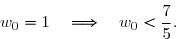
Initialisation : Montrons que la propriété est vraie pour n = 0, soit que
C'est une évidence car
Donc l'initialisation est vraie.
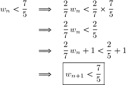
Hérédité : Montrons que si pour un nombre naturel n fixé, la propriété est vraie au rang n , alors elle est encore vraie au rang (n +1).
Montrons donc que si pour un nombre naturel n fixé, , alors
En effet,
L'hérédité est vraie.
Puisque l'initialisation et l'hérédité sont vraies, nous avons montré par récurrence que pour tout entier naturel
2. a) Montrons que est une suite croissante.
Pour tout
Nous en déduisons que est une suite croissante.
2. b) La suite est croissante et majorée par Cette suite est donc convergente.
3 points
exercice 2
Soit la suite définie par :
et
pour tout
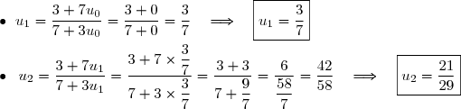
1. Calculons et
2. On pose pour tout de
2. a) Calculons
2. b) Montrons que est une suite géométrique de raison
Par conséquent, est une suite géométrique de raison
2. c) Le terme général de la suite est .
Donc, pour tout de , soit
3. a) Nous devons montrer que
3. b) Sur base des questions 2. c) et 3. a), nous déduisons que pour tout de
3. c) Nous devons calculer
Nous savons que
Dès lors,
1 point
exercice 3
Soit et deux événements indépendants tels que et
Nous devons calculer
Les événements et sont indépendants.
Donc
Nous obtenons alors :
3 points
exercice 4
La répartition des jetons est donnée par le tableau suivant :
1. a) Parmi les 100 jetons, 64 d'entre eux sont blancs. La probabilité que le jeton soit de couleur blanche est
1. b) Parmi les 100 jetons, 34 d'entre eux portent le chiffre 2. La probabilité que le jeton porte le chiffre 2 est
1. c) Parmi les 100 jetons, 14 d'entre eux portent le chiffre 2 et sont de couleur blanche. La probabilité que le jeton porte le chiffre 2 et soit de couleur blanche est
2. Parmi les 64 jetons blancs, 14 d'entre eux portent le chiffre 2. La probabilité que le jeton porte le chiffre 2 sachant qu'il est de couleur blanche est
Remarque : Nous aurions pu trouver le même résultat par le calcul :
3. On considère la variable aléatoire qui est égale au chiffre porté par le jeton.
3. a) Tableau complété.
3. b) Nous devons calculer l'espérance mathématique de
2,5 points
exercice 5
1. Deux calculs de limites.
Calculons
Calculons
D'une part,
D'autre part,
Par conséquent,
2.Calculons
D'où
Calculons
D'où
8,5 points
exercice 6
On considère la fonction numérique de la variable réelle définie sur par :
1. a) Nous devons calculer
Par conséquent,
Nous en déduisons que la courbe admet une asymptote horizontale en + d'équation :
1. b) Nous devons calculer et
Calculons
Par conséquent,
Calculons
Nous savons que .
Par conséquent,
Nous en déduisons que la courbe admet une branche parabolique de direction l'axe des ordonnées au voisinage de -.
2. a) Calculons pour tout réel
Pour tout réel
2. b) Étudions le signe de et dressons le tableau de variations de
Puisque l'exponentielle est strictement positive pour tout réel , le signe de est le signe de
Dressons le tableau de variations de
2. b) Déterminons l'équation de la tangente à au point d'abscisse 0.
L'équation de cette tangente est de la forme soit de la forme
Or
D'où une équation de la tangente à au point d'abscisse 0 est
3. Calculons pour tout réel
Montrons que la courbe admet un point d'inflexion.
Étudions le signe de
Puisque l'exponentielle est strictement positive pour tout réel , le signe de est le signe de
Nous observons que s'annule et change de signe en 2.
Dès lors, la courbe admet un point d'inflexion d'abscisse 2.
4. Dans la figure ci-dessous, est la courbe représentative de et la droite d'équation : dans le repère orthonormé
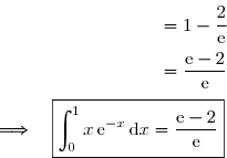
4. a) Montrons que
Calculons
4. b) Nous devons en déduire l'aire de la partie hachurée.
La partie hachurée correspond à la portion du plan comprise entre la droite , la courbe , les droites d'équations et
De plus, nous remarquons que pour tout
Donc sur l'intervalle [0 ; 1], la droite est au-dessus de la courbe
Dès lors,
Publié par malou/Panter
le
ceci n'est qu'un extrait
Pour visualiser la totalité des cours vous devez vous inscrire / connecter (GRATUIT) Inscription Gratuitese connecter
Merci à Hiphigenie / Panter pour avoir contribué à l'élaboration de cette fiche
Désolé, votre version d'Internet Explorer est plus que périmée ! Merci de le mettre à jour ou de télécharger Firefox ou Google Chrome pour utiliser le site. Votre ordinateur vous remerciera !
_{n\in\N} }) la suite définie par :
la suite définie par :
 et
et  pour tout
 pour
tout
pour
tout  de
de 

 , alors


-w_n \\\overset{ { \white{ . } } } { \phantom{w_{n+1}-w_n}=1-\dfrac57\,w_n})
\times\dfrac75 \\\overset{ { \white{ . } } } {\phantom{\text{Or }\;w_n<\dfrac75}\quad\Longrightarrow\quad -\dfrac57\,w_n>-1} \\\overset{ { \white{ . } } } {\phantom{\text{Or }\;w_n<\dfrac75}\quad\Longrightarrow\quad 1-\dfrac57\,w_n>0} \\\overset{ { \phantom{ . } } } {\phantom{\text{Or }\;w_n<\dfrac75}\quad\Longrightarrow\quad \boxed{w_{n+1}-w_n>0}})
_{n\in\N} }) est croissante et majorée par
est croissante et majorée par 
 Cette suite
 _{n\in\N} }) la suite définie par :
la suite définie par :
 et
et 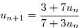 pour tout
  et
et 
 pour tout

_{n\in\N} }) est une suite géométrique de raison
est une suite géométrique de raison 
-(3+7u_n)}{7+3u_n}}{\frac{(7+3u_n)+(3+7u_n)}{7+3u_n}}=\dfrac{7+3u_n-3-7u_n}{7+3u_n+3+7u_n} \\\overset{ { \white{ . } } } { \phantom{v_{n+1}}=\dfrac{4-4u_n}{10+10u_n} =\dfrac{4(1-u_n)}{10(1+u_n)} =\dfrac{2(1-u_n)}{5(1+u_n)} =\dfrac{2}{5}\times\dfrac{1-u_n}{1+u_n} =\dfrac{2}{5}\times v_n } \\\\\Longrightarrow\quad\boxed{\forall\,n\in\N,\;v_{n+1}=\dfrac25\,v_n})

 .
.^{n} }) , soit
, soit ^{n}}\,. })

=1-u_n \\\phantom{v_n=\dfrac{1-u_n}{1+u_n}}\quad\Longleftrightarrow\quad v_n+u_n\,v_n=1-u_n \\\phantom{v_n=\dfrac{1-u_n}{1+u_n}}\quad\Longleftrightarrow\quad u_n+u_n\,v_n=1-v_n \\\phantom{v_n=\dfrac{1-u_n}{1+u_n}}\quad\Longleftrightarrow\quad u_n\,(1+v_n)=1-v_n \\\phantom{v_n=\dfrac{1-u_n}{1+u_n}}\quad\Longleftrightarrow\quad \boxed{u_n=\dfrac{1-v_n}{1+v_n}})

^{n}}\end{matrix}\right.\quad\Longrightarrow\quad \boxed{u_n=\dfrac{1-\left(\dfrac25\right)^{n}}{1+\left(\dfrac25\right)^{n}}})

^{n}=0. })
^{n}}{1+\left(\dfrac25\right)^{n}}=\dfrac{1-0}{1+0}\quad\Longrightarrow\quad\boxed{\lim\limits_{n\to+\infty}u_n=1} })
 et
et  deux événements indépendants tels que
 =\dfrac12 }) et
et =\dfrac58. })
. })
=p(A)\times p(B). })
=p(A)+p(B)-p(A\cap B)\quad\Longleftrightarrow\quad p(A\cup B)=p(A)+p(B)-p(A)\times p( B) \\\overset{ { \white{ . } } } {\phantom{p(A\cup B)=p(A)+p(B)-p(A\cap B)}\quad\Longleftrightarrow\quad \dfrac58=\dfrac12+p(B)-\dfrac12\times p(B) } \\\overset{ { \white{ . } } } {\phantom{p(A\cup B)=p(A)+p(B)-p(A\cap B)}\quad\Longleftrightarrow\quad \dfrac58-\dfrac12=\dfrac12\times p(B) } \\\overset{ { \white{ . } } } {\phantom{p(A\cup B)=p(A)+p(B)-p(A\cap B)}\quad\Longleftrightarrow\quad \dfrac18=\dfrac12\times p(B) } \\\overset{ { \phantom{ . } } } {\phantom{p(A\cup B)=p(A)+p(B)-p(A\cap B)}\quad\Longleftrightarrow\quad \boxed{p(B)=\dfrac14 }})

 qui est égale au chiffre porté par le jeton.
&&\dfrac{66}{100}&&&\dfrac{34}{100}&\\&&&&&&\\\hline \end{array} )
 }) de
de 
=1\times\dfrac{66}{100}+2\times\dfrac{34}{100}=\dfrac{134}{100}=\dfrac{67}{50}\quad\Longrightarrow\quad\boxed{E(X)=\dfrac{67}{50}}\,.)
 Calculons
 }.)
=+\infty}\end{matrix}\right. \\\\\\\phantom{WWWWWWW}\quad\Longrightarrow\quad\boxed{\lim\limits_{\overset{x\to0}{x>0}}\,\left(\dfrac{1}{x}-\ln x\right)=+\infty})
}.)
=\lim\limits_{\overset{x\to0}{x>0}}\,\dfrac{1}{x}\left(1+x\ln x\right). })
}\end{matrix}\right. \quad\Longrightarrow\quad\left\lbrace\begin{matrix}\lim\limits_{\overset{x\to0}{x>0}}\;\dfrac{1}{x}=+\infty\\\overset{ { \white{ . } } } { \lim\limits_{\overset{x\to0}{x>0}}\,(1+x\ln x)=1}\end{matrix}\right. \\\\\\\phantom{WWWWWWWWWWWWWWWWW}\quad\Longrightarrow\quad\lim\limits_{\overset{x\to0}{x>0}}\,\dfrac{1}{x}\left(1+x\ln x\right)=+\infty)
=+\infty} })

\quad\text{où }f\text{ est définie par }f(x)=\ln x} \\\overset{ { \white{ . } } } {\phantom{\lim\limits_{x\to1}\,\dfrac{\ln x}{x-1}}=1\quad\text{car }f'(x)=\dfrac1x\Longrightarrow f'(1)=\dfrac11=1})

}\,.)
=\lim\limits_{x\to1}\,\left(\dfrac{\ln x}{x-1}\times x\right) \\\phantom{\lim\limits_{x\to1}\,\dfrac{x}{x-1}\times \ln x))))}=1\times1 \\\phantom{\lim\limits_{x\to1}\,\dfrac{x}{x-1}\times \ln x)))}=1)
=1} })
 de la variable réelle
  définie sur
  par :
par : =1-\dfrac{x}{\text e^x}. })
. })
=\lim\limits_{x\to+\infty}\left(-x\,\text e^{-x}\right) \\\phantom{\lim\limits_{x\to+\infty}\left(-\dfrac{x}{\text e^x}\right)}=\lim\limits_{X\to-\infty}X\,\text e^{X}\quad\text{où }\;X=-x \\\phantom{\lim\limits_{x\to+\infty}\left(-\dfrac{x}{\text e^x}\right)}=0\quad(\text{croissances comparées}) \\\\\Longrightarrow\quad \lim\limits_{x\to+\infty}\left(1-\dfrac{x}{\text e^x}\right)=1)
=1} })
}) admet une asymptote horizontale en +
admet une asymptote horizontale en + d'équation :
 }) et
et }{x}. })
}\,.)
=+\infty)
=+\infty} })
}{x}}\,.)
}{x}=\dfrac1x-\dfrac{1}{\text e^x}}) .
.=-\infty})
}{x}=-\infty} })
 }) pour tout réel
pour tout réel 

=\left(1-\dfrac{x}{\text e^x}\right)' \\\overset{ { \white{ . } } } { \phantom{f'(x)}=-\left(\dfrac{x}{\text e^x}\right)'} \\\overset{ { \white{ . } } } { \phantom{f'(x)}=-\left(\dfrac{x'\times\text e^x-x\times(\text e^x)'}{(\text e^x)^2}\right)} \\\overset{ { \white{ . } } } { \phantom{f'(x)}=-\left(\dfrac{1\times\text e^x-x\times\text e^x}{\text e^{2x}}\right)})
}=-\left(\dfrac{\text e^x-x\,\text e^x}{\text e^{2x}}\right)} \\\overset{ { \white{ . } } } { \phantom{f'(x)}=-\left(\dfrac{\text e^x(1-x)}{\text e^{2x}}\right)} \\\overset{ { \white{ . } } } { \phantom{f'(x)}=-\left(\dfrac{1-x}{\text e^{x}}\right)} \\\overset{ { \phantom{ . } } } { \phantom{f'(x)}=\dfrac{x-1}{\text e^{x}}} \\\\\Longrightarrow\quad\boxed{\forall\,x\in\R,\;f'(x)=\dfrac{x-1}{\text e^{x}}})

. })
&&-&-&0&+&+&\\&&&&&&&\\\hline \end{array} )
&&-&-&0&+&+&\\&&&&&&&\\\hline&+\infty&&&&&&1\\f(x)&&\searrow&\searrow&&\nearrow&\nearrow&\\&&&&1-\dfrac{1}{\text e}&&&\\\hline \end{array} )
 }) au point d'abscisse 0.
au point d'abscisse 0.(x-0)+f(0), }) soit de la forme
soit de la forme x+f(0)} })
=1-\dfrac{x}{\text e^x}\\\overset{ { \white{ . } } } { f'(x)=\dfrac{x-1}{\text e^x}}\end{matrix}\right.\quad\Longrightarrow\quad\left\lbrace\begin{matrix}f(0)=1-\dfrac{0}{1}\\\overset{ { \white{ . } } } { f'(0)=\dfrac{0-1}{1}}\end{matrix}\right.\quad\Longrightarrow\quad\left\lbrace\begin{matrix}f(0)=1\\\overset{ { \white{ . } } } { f'(0)=-1}\end{matrix}\right.)

 }) pour tout réel
pour tout réel =\left(\dfrac{x-1}{\text e^{x}}\right)' \\\overset{ { \white{ . } } } { \phantom{f''(x)}=\dfrac{(x-1)'\times\text e^{x}-(x-1)\times(\text e^{x})'}{(\text e^{x})^2}} \\\overset{ { \white{ . } } } { \phantom{f''(x)}=\dfrac{1\times\text e^{x}-(x-1)\times\text e^{x}}{\text e^{2x}}} \\\overset{ { \white{ . } } } { \phantom{f''(x)}=\dfrac{\text e^{x}-(x-1)\,\text e^{x}}{\text e^{2x}}})
![\\\overset{ { \white{ . } } } { \phantom{f''(x)}=\dfrac{\text e^{x}[1-(x-1)]}{\text e^{2x}}} \\\overset{ { \white{ . } } } { \phantom{f''(x)}=\dfrac{1-x+1}{\text e^{x}}} \\\overset{ { \phantom{ . } } } { \phantom{f''(x)}=\dfrac{2-x}{\text e^{x}}} \\\\\Longrightarrow\quad\boxed{\forall\,x\in\R,\;f''(x)=\dfrac{2-x}{\text e^{x}}}](https://latex.ilemaths.net/latex-0.tex?\\\overset{ { \white{ . } } } { \phantom{f''(x)}=\dfrac{\text e^{x}[1-(x-1)]}{\text e^{2x}}} \\\overset{ { \white{ . } } } { \phantom{f''(x)}=\dfrac{1-x+1}{\text e^{x}}} \\\overset{ { \phantom{ . } } } { \phantom{f''(x)}=\dfrac{2-x}{\text e^{x}}} \\\\\Longrightarrow\quad\boxed{\forall\,x\in\R,\;f''(x)=\dfrac{2-x}{\text e^{x}}})
. })
&&+&+&0&-&-&\\&&&&&&&\\\hline \end{array} )
}) s'annule et change de signe en 2.
s'annule et change de signe en 2. et
et }) la droite d'équation :
la droite d'équation :  dans le repère orthonormé
 .})
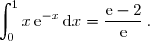

![\underline{\text{Formule de l'intégrale par parties}}\ :\ {\blue{\displaystyle\int_0^{1}u(x)v'(x)\,\text{d}x=\left[\overset{}{u(x)v(x)}\right]\limits_0^{1}- \displaystyle\int\limits_0^{1}u'(x)v(x)\,\text{d}x}}. \\ \\ \left\lbrace\begin{matrix}u(x)=x\quad\Longrightarrow\quad u'(x)=1 \\\\v'(x)=\text e^{-x}\phantom{}\quad\Longrightarrow\quad v(x)=-\text e^{-x}\end{matrix}\right.](https://latex.ilemaths.net/latex-0.tex?\underline{\text{Formule de l'intégrale par parties}}\ :\ {\blue{\displaystyle\int_0^{1}u(x)v'(x)\,\text{d}x=\left[\overset{}{u(x)v(x)}\right]\limits_0^{1}- \displaystyle\int\limits_0^{1}u'(x)v(x)\,\text{d}x}}. \\ \\ \left\lbrace\begin{matrix}u(x)=x\quad\Longrightarrow\quad u'(x)=1 \\\\v'(x)=\text e^{-x}\phantom{}\quad\Longrightarrow\quad v(x)=-\text e^{-x}\end{matrix}\right.)
![\text{Dès lors }\;\overset{ { \white{ . } } } { \displaystyle\int_{0}^{1} x\,\text e^{-x}\,\text{d}x=\left[\overset{}{-x\,\text e^{-x}}\right]_0^{1}-\displaystyle\int_0^{1}1\times(-\text{e}^{-x})\,\text{d}x} \\\overset{ { \white{ . } } } {\phantom{WWWWWWWW}=\left[\overset{}{-x\,\text e^{-x}}\right]_0^{1}-\displaystyle\int_0^{1}-\text{e}^{-x}\,\text{d}x} \\\overset{ { \phantom{ . } } } {\phantom{WWWWWWWW}=\left[\overset{}{-x\,\text e^{-x}}\right]_0^{1}-\left[\overset{}{\text e^{-x}}\right]_0^{1}} \\\overset{ { \phantom{ . } } } {\phantom{WWWWWWWW}=(-\,\text e^{-1}-0)-(\text e^{-1}-\text e^0)} \\\overset{ { \white{ . } } } {\phantom{WWWWWWWW}=-\,\text e^{-1}-\text e^{-1}+1} \\\overset{ { \phantom{ . } } } { \phantom{WWWWWWWW}=-2\,\text e^{-1}+1}](https://latex.ilemaths.net/latex-0.tex?\text{Dès lors }\;\overset{ { \white{ . } } } { \displaystyle\int_{0}^{1} x\,\text e^{-x}\,\text{d}x=\left[\overset{}{-x\,\text e^{-x}}\right]_0^{1}-\displaystyle\int_0^{1}1\times(-\text{e}^{-x})\,\text{d}x} \\\overset{ { \white{ . } } } {\phantom{WWWWWWWW}=\left[\overset{}{-x\,\text e^{-x}}\right]_0^{1}-\displaystyle\int_0^{1}-\text{e}^{-x}\,\text{d}x} \\\overset{ { \phantom{ . } } } {\phantom{WWWWWWWW}=\left[\overset{}{-x\,\text e^{-x}}\right]_0^{1}-\left[\overset{}{\text e^{-x}}\right]_0^{1}} \\\overset{ { \phantom{ . } } } {\phantom{WWWWWWWW}=(-\,\text e^{-1}-0)-(\text e^{-1}-\text e^0)} \\\overset{ { \white{ . } } } {\phantom{WWWWWWWW}=-\,\text e^{-1}-\text e^{-1}+1} \\\overset{ { \phantom{ . } } } { \phantom{WWWWWWWW}=-2\,\text e^{-1}+1})
 de la partie hachurée.
 et
et 
![\overset{ { \white{ . } } } { x\in[0\;;\;1],\;1-f(x)=1-\left(1-\dfrac{x}{\text e^x}\right)=\dfrac{x}{\text e^x}>0. }](https://latex.ilemaths.net/latex-0.tex?\overset{ { \white{ . } } } { x\in[0\;;\;1],\;1-f(x)=1-\left(1-\dfrac{x}{\text e^x}\right)=\dfrac{x}{\text e^x}>0. })
.})
)\,\text{d}x} \\\overset{ { \phantom{ . } } }{\phantom{A}= \displaystyle\int_{0}^{1} \Big(1-\left(1-\dfrac{x}{\text e^x}\right)\Big)\,\text{d}x} \\\overset{ { \phantom{ . } } } { \phantom{A}=\displaystyle\int_{0}^{1} \dfrac{x}{\text e^x}\,\text{d}x} \\\phantom{A}=\overset{ { \phantom{ . } } } { \displaystyle\int_{0}^{1} x\,\text e^{-x}\,\text{d}x} \\\phantom{A}=\overset{ { \phantom{ . } } } { \dfrac{\text e-2}{\text e}\;\text{u.a.}} \\\\\Longrightarrow \boxed{\mathscr{A}= \dfrac{\text e-2}{\text e}\;\text{u.a.}\approx0,26\;\text{u.a.}}) Publié par malou/Panter
le
Publié par malou/Panter
le
 Voir la correction
 forum de terminale